Dispersive Shift of a Transmon–Resonator System with Pymablock
Required extras
This notebook needs the
modelsandpymablockextras:uv add "qpdk[models,pymablock]" # or, from a checkout of this repository: uv sync --extra models --extra pymablock # or with pip: pip install "qpdk[models,pymablock]"See the extras reference for what each extra installs.
This notebook demonstrates how to use pymablock Araya Day et al. (2025) to compute the dispersive shift of a readout resonator coupled to a transmon qubit, and how to translate the resulting Hamiltonian parameters into physical layout parameters using qpdk.
Background
In circuit quantum electrodynamics (cQED), the state of a transmon qubit is typically measured via the dispersive readout technique Blais et al. (2021). The qubit is detuned from a readout resonator, and the qubit-state-dependent frequency shift of the resonator—the dispersive shift \(\chi\)—allows non-destructive measurement of the qubit state.
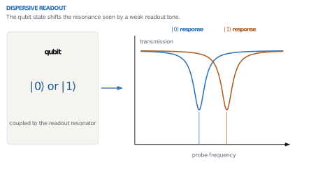
The two response frequencies differ by \(\chi\) under the convention used below; the sketch shows the separation qualitatively, without assigning its sign.
The full transmon–resonator Hamiltonian (without the rotating-wave approximation) reads:
where \(\omega_\text{t}\) is the transmon frequency, \(\alpha\) its anharmonicity, \(\omega_\text{r}\) the resonator frequency, and \(g\) the coupling strength.
Treating \(g\) as a perturbative parameter, pymablock computes the effective (block-diagonal) Hamiltonian to any desired order, from which we extract \(\chi\).
??? note "Show code"
```
import jax.numpy as jnp
import polars as pl
import scipy
import sympy
from IPython.display import Math, display
from matplotlib import pyplot as plt
from pymablock import block_diagonalize
from pymablock.number_ordered_form import NumberOperator
from sympy.physics.quantum.boson import BosonOp

from qpdk import PDK
from qpdk.helper import display_dataframe
from qpdk.models.constants import c_0
from qpdk.models.cpw import cpw_parameters

PDK.activate()

from qpdk.models.perturbation import (
    dispersive_shift,
    dispersive_shift_to_coupling,
    ej_ec_to_frequency_and_anharmonicity,
    measurement_induced_dephasing,
    purcell_decay_rate,
    resonator_linewidth_from_q,
    transmon_resonator_hamiltonian,
)
from qpdk.models.qubit import (
    coupling_strength_to_capacitance,
    ec_to_capacitance,
    ej_to_inductance,
)
from qpdk.models.resonator import resonator_frequency
```
Building the Hamiltonian
We first construct the Hamiltonian symbolically using bosonic operators from
SymPy, following the conventions of pymablock. The helper
transmon_resonator_hamiltonian returns the unperturbed part \(H_0\) and the
perturbation \(H_\text{p}\) together with the symbolic parameters.
??? note "Show code"
```
def display_eq(title: str, expr: sympy.Basic) -> None:
    """Display a named symbolic expression."""
    display(sympy.Eq(sympy.Symbol(title), expr, evaluate=False))
```
H_0, H_p, (omega_t, omega_r, alpha, g) = transmon_resonator_hamiltonian()

display_eq("H_{0}", H_0)
display_eq("H_{p}", H_p)
Effective Hamiltonian
Using block_diagonalize on the full second-quantized Hamiltonian,
pymablock returns the effective Hamiltonian as a function of the
number operators \(N_{a_\text{t}}\) and \(N_{a_\text{r}}\). The dispersive shift is:
where \(E^{(2)}_{ij}\) is the second-order energy correction for \(i\) transmon excitations and \(j\) resonator excitations.
For details on pymablock and the block-diagonalization procedure, see pymablock documentation.
H_tilde, U, U_adj = block_diagonalize(H_0 + H_p, symbols=[g])

E_eff = H_tilde[0, 0, 2]
display_eq("E_{eff}^{(2)}", E_eff)
# Evaluate for specific occupation numbers
a_t_op = BosonOp("a_t")
a_r_op = BosonOp("a_r")
N_a_t = NumberOperator(a_t_op)
N_a_r = NumberOperator(a_r_op)

E_00 = E_eff.subs({N_a_t: 0, N_a_r: 0})
E_01 = E_eff.subs({N_a_t: 0, N_a_r: 1})
E_10 = E_eff.subs({N_a_t: 1, N_a_r: 0})
E_11 = E_eff.subs({N_a_t: 1, N_a_r: 1})

chi_sym = E_11 - E_10 - E_01 + E_00

# Convert from pymablock's NumberOrderedForm to a standard sympy expression
if hasattr(chi_sym, "as_expr"):
    chi_sym = chi_sym.as_expr()

display_eq(r"\chi", chi_sym)
The full expression (including counter-rotating terms) is:
Numerical Evaluation
We now evaluate \(\chi\) for realistic transmon parameters. We start from the Josephson energy \(E_\text{J}\) and charging energy \(E_\text{C}\), which fully determine the transmon frequency and anharmonicity in the transmon regime (\(E_\text{J} \gg E_\text{C}\)):
# Hamiltonian parameters (in GHz)
EJ = 20.0  # Josephson energy
EC = 0.2  # Charging energy
omega_r_val = 7.0  # Resonator frequency
g_val = 0.1  # Coupling strength

# Derived transmon parameters
omega_t_val, alpha_val = ej_ec_to_frequency_and_anharmonicity(EJ, EC)

display(
    Math(rf"""
\textbf{{Hamiltonian Parameters:}} \\
E_\text{{J}} = {EJ:.1f}\,\text{{GHz}}, \quad
E_\text{{C}} = {EC:.1f}\,\text{{GHz}} \\
\omega_\text{{t}} = \sqrt{{8 E_\text{{J}} E_\text{{C}}}} - E_\text{{C}} = {omega_t_val:.3f}\,\text{{GHz}} \\
\alpha \approx E_\text{{C}} = {alpha_val:.1f}\,\text{{GHz}} \\
\omega_\text{{r}} = {omega_r_val:.1f}\,\text{{GHz}} \\
g = {g_val:.1f}\,\text{{GHz}} \\
\Delta = \omega_\text{{t}} - \omega_\text{{r}} = {omega_t_val - omega_r_val:.3f}\,\text{{GHz}}
""")
)

# Compute dispersive shift using the analytical formula from perturbation.py
chi_numerical = dispersive_shift(omega_t_val, omega_r_val, alpha_val, g_val)

display(
    Math(
        rf"\chi = {chi_numerical * 1e3:.3f}\,\text{{MHz}} "
        rf"= {chi_numerical * 1e6:.1f}\,\text{{kHz}}"
    )
)

# Verify against the symbolic expression
chi_check = float(
    chi_sym.subs(
        {
            omega_t: omega_t_val,
            omega_r: omega_r_val,
            alpha: alpha_val,
            g: g_val,
        }
    )
)
print(
    f"Symbolic evaluation: χ = {chi_check * 1e3:.3f} MHz "
    f"(difference: {abs(chi_numerical - chi_check):.2e} GHz)"
)
Symbolic evaluation: χ = 1.513 MHz (difference: 8.28e-07 GHz)
Dispersive Shift vs. Coupling Strength
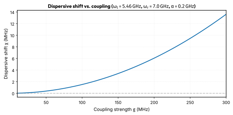
We now sweep the coupling strength \(g\) to see how the dispersive shift depends on it. The quadratic dependence \(\chi \propto g^2\) is clearly visible.
g_sweep = jnp.linspace(0.01, 0.3, 200)
chi_sweep = jnp.array(
    [dispersive_shift(omega_t_val, omega_r_val, alpha_val, gi) for gi in g_sweep]
)

fig, ax = plt.subplots(figsize=(8, 4))
ax.plot(g_sweep * 1e3, chi_sweep * 1e3, "-", linewidth=2)
ax.axhline(0, color="gray", linestyle="--", alpha=0.5)
ax.set_xlabel("Coupling strength $g$ (MHz)")
ax.set_ylabel(r"Dispersive shift $\chi$ (MHz)")
ax.set_title(
    rf"Dispersive shift vs. coupling ($\omega_\text{{t}} = {omega_t_val:.2f}\,\text{{GHz}}$, "
    rf"$\omega_\text{{r}} = {omega_r_val:.1f}\,\text{{GHz}}$, $\alpha = {alpha_val:.1f}\,\text{{GHz}}$)"
)
ax.grid(True, alpha=0.3)
fig.tight_layout()
plt.show()
Design Workflow: From Hamiltonian to Layout Parameters
The purpose of computing \(\chi\) analytically is to design a qubit–resonator system with a target dispersive shift. The workflow is:
- Choose target \(\chi\) based on readout speed requirements
- Select \(\omega_\text{t}\), \(\omega_\text{r}\), \(\alpha\) from qubit design goals
- Determine \(g\) from target \(\chi\) using (3)
- Convert to circuit parameters (\(C_\Sigma\), \(L_\text{J}\), \(C_\text{c}\)) using qpdk helpers
- Convert to layout parameters (resonator length, capacitor geometry)
Step 1–3: From target \(\chi\) to coupling \(g\)
# Design targets
chi_target_mhz = -1.0  # Target dispersive shift in MHz
chi_target = chi_target_mhz * 1e-3  # Convert to GHz

# Qubit and resonator parameters
EJ_design = 20.0  # GHz
EC_design = 0.2  # GHz
omega_r_design = 7.0  # GHz

omega_t_design, alpha_design = ej_ec_to_frequency_and_anharmonicity(
    EJ_design, EC_design
)

# Compute required coupling strength
g_design = dispersive_shift_to_coupling(
    chi_target, omega_t_design, omega_r_design, alpha_design
)

# Verify: compute χ with the found g
chi_verify = dispersive_shift(omega_t_design, omega_r_design, alpha_design, g_design)

display(
    Math(rf"""
\textbf{{Step 1–3: Hamiltonian Design}} \\
\text{{Target:}}\quad \chi = {chi_target_mhz:.1f}\,\text{{MHz}} \\
\text{{Required coupling:}}\quad g = {g_design * 1e3:.1f}\,\text{{MHz}} \\
\text{{Verification:}}\quad \chi(g) = {chi_verify * 1e3:.3f}\,\text{{MHz}}
""")
)
Step 4: Convert to circuit parameters
Using the qpdk helper functions, we convert the Hamiltonian parameters
to circuit parameters:
- Total qubit capacitance \(C_\Sigma\) from \(E_\text{C}\) via ec_to_capacitance
- Josephson inductance \(L_\text{J}\) from \(E_\text{J}\) via ej_to_inductance
- Coupling capacitance \(C_\text{c}\) from \(g\) via coupling_strength_to_capacitance
# Total qubit capacitance
C_sigma = float(ec_to_capacitance(EC_design))

# Josephson inductance
L_J = float(ej_to_inductance(EJ_design))

# For coupling capacitance, we need the resonator capacitance.
# First, determine resonator length for the target frequency.
ep_eff, z0 = cpw_parameters(width=10, gap=6)


def _resonator_objective(length: float) -> float:
    """Minimize the squared frequency error.

    Returns:
        The squared error between the calculated and target frequency.
    """
    freq = resonator_frequency(
        length=length,
        epsilon_eff=float(jnp.real(ep_eff)),
        is_quarter_wave=True,
    )
    return (freq - omega_r_design * 1e9) ** 2


result = scipy.optimize.minimize(_resonator_objective, 4000.0, bounds=[(1000, 20000)])
resonator_length = result.x[0]

# Total resonator capacitance from CPW impedance and phase velocity
C_r = 1 / jnp.real(z0 * (c_0 / jnp.sqrt(ep_eff))) * resonator_length * 1e-6  # F

# Coupling capacitance
C_c = float(
    coupling_strength_to_capacitance(
        g_ghz=g_design,
        c_sigma=C_sigma,
        c_r=C_r,
        f_q_ghz=omega_t_design,
        f_r_ghz=omega_r_design,
    )
)

display(
    Math(rf"""
\textbf{{Step 4: Circuit Parameters}} \\
C_\Sigma = {C_sigma * 1e15:.1f}\,\text{{fF}} \\
L_\text{{J}} = {L_J * 1e9:.2f}\,\text{{nH}} \\
C_\text{{r}} = {C_r * 1e15:.1f}\,\text{{fF}} \\
C_\text{{c}} = {C_c * 1e15:.2f}\,\text{{fF}}
""")
)
Step 5: Layout parameters
The circuit parameters map directly to layout dimensions:
f_resonator_achieved = resonator_frequency(
    length=resonator_length,
    epsilon_eff=float(jnp.real(ep_eff)),
    is_quarter_wave=True,
)

display(
    Math(rf"""
\textbf{{Step 5: Layout Parameters}} \\
\text{{Resonator length:}}\quad l = {resonator_length:.0f}\,\text{{µm}} \\
\text{{Resonator CPW width:}}\quad w = 10\,\text{{µm}}, \quad
\text{{gap}} = 6\,\text{{µm}} \\
\text{{Resonator frequency achieved:}}\quad
f_\text{{r}} = {f_resonator_achieved / 1e9:.3f}\,\text{{GHz}}
""")
)
Readout System Design Considerations
A complete readout design also requires considering the resonator linewidth \(\kappa\), the Purcell decay rate, and the measurement-induced dephasing.
# Resonator quality factor and linewidth
Q_ext = 10_000  # External quality factor
kappa = resonator_linewidth_from_q(omega_r_design, Q_ext)

# Purcell decay rate
gamma_purcell = purcell_decay_rate(g_design, omega_t_design, omega_r_design, kappa)
T_purcell = 1 / (gamma_purcell * 1e9) if gamma_purcell > 0 else float("inf")

# Measurement-induced dephasing
n_bar = 5.0  # Mean photon number during readout
gamma_phi = measurement_induced_dephasing(chi_verify, kappa, n_bar)

# SNR estimate: the signal-to-noise ratio scales as χ/κ
chi_over_kappa = abs(chi_verify) / kappa

display(
    Math(rf"""
\textbf{{Readout System Parameters:}} \\
Q_\text{{ext}} = {Q_ext:,} \\
\kappa = \omega_\text{{r}} / Q_\text{{ext}} = {kappa * 1e6:.1f}\,\text{{kHz}} \\
\gamma_\text{{Purcell}} = \kappa (g/\Delta)^2
  = {gamma_purcell * 1e6:.2f}\,\text{{kHz}}
  \quad \Rightarrow \quad T_\text{{Purcell}}
  = {T_purcell * 1e6:.0f}\,\text{{µs}} \\
\Gamma_\phi(\bar{{n}}={n_bar:.0f})
  = 8\chi^2 \bar{{n}} / \kappa
  = {gamma_phi * 1e6:.2f}\,\text{{kHz}} \\
|\chi| / \kappa = {chi_over_kappa:.1f}
  \quad (\text{{want}} \gtrsim 1 \text{{ for high-fidelity readout}})
""")
)
Summary: Complete Design Table
The table below summarises the full design flow from Hamiltonian parameters to layout parameters, with the dispersive shift as the central design target.
data = [
    ("Target", "Target dispersive shift $\\chi$", f"{chi_target_mhz:.1f}", "MHz"),
    ("Hamiltonian", "$E_\\text{J}$", f"{EJ_design:.1f}", "GHz"),
    ("Hamiltonian", "$E_\\text{C}$", f"{EC_design:.1f}", "GHz"),
    ("Hamiltonian", "$\\omega_\\text{t}$", f"{omega_t_design:.3f}", "GHz"),
    ("Hamiltonian", "$\\alpha$", f"{alpha_design:.1f}", "GHz"),
    ("Hamiltonian", "$\\omega_\\text{r}$", f"{omega_r_design:.1f}", "GHz"),
    ("Hamiltonian", "$g$", f"{g_design * 1e3:.1f}", "MHz"),
    ("Circuit", "$C_\\Sigma$", f"{C_sigma * 1e15:.1f}", "fF"),
    ("Circuit", "$L_\\text{J}$", f"{L_J * 1e9:.2f}", "nH"),
    ("Circuit", "$C_\\text{r}$", f"{C_r * 1e15:.1f}", "fF"),
    ("Circuit", "$C_\\text{c}$", f"{C_c * 1e15:.2f}", "fF"),
    ("Layout", "Resonator length", f"{resonator_length:.0f}", "µm"),
    ("Layout", "Resonator CPW width", "10", "µm"),
    ("Layout", "Resonator CPW gap", "6", "µm"),
    ("Layout", "Resonator freq", f"{f_resonator_achieved / 1e9:.3f}", "GHz"),
    ("Readout", "$Q_{\\text{ext}}$", f"{Q_ext:,}", ""),
    ("Readout", "$\\kappa$", f"{kappa * 1e6:.1f}", "kHz"),
    ("Readout", "$T_{\\text{Purcell}}$", f"{T_purcell * 1e6:.0f}", "µs"),
    ("Readout", "$|\\chi|/\\kappa$", f"{chi_over_kappa:.1f}", ""),
]

df = pl.DataFrame(data, schema=["Category", "Parameter", "Value", "Unit"], orient="row")

display_dataframe(df)
| Category | Parameter | Value | Unit |
|---|---|---|---|
| Target | Target dispersive shift χ | -1.0 | MHz |
| Hamiltonian | EJ | 20.0 | GHz |
| Hamiltonian | EC | 0.2 | GHz |
| Hamiltonian | ωt | 5.457 | GHz |
| Hamiltonian | α | 0.2 | GHz |
| Hamiltonian | ωr | 7.0 | GHz |
| Hamiltonian | g | 82.0 | MHz |
| Circuit | CΣ | 96.9 | fF |
| Circuit | LJ | 8.17 | nH |
| Circuit | Cr | 724.2 | fF |
| Circuit | Cc | 7.03 | fF |
| Layout | Resonator length | 4348 | µm |
| Layout | Resonator CPW width | 10 | µm |
| Layout | Resonator CPW gap | 6 | µm |
| Layout | Resonator freq | 7.000 | GHz |
| Readout | Qext | 10,000 | |
| Readout | κ | 700.0 | kHz |
| Readout | TPurcell | 506 | µs |
| Readout | |χ|/κ | 1.5 |
References
- Araya Day, Isidora and Miles, Sebastian and Kerstens, Hugo K. and Varjas, Daniel and Akhmerov, Anton R., Pymablock: An Algorithm and a Package for Quasi-Degenerate Perturbation Theory, SciPost Physics Codebases, 2025. doi:10.21468/SciPostPhysCodeb.50
- Blais, Alexandre and Grimsmo, Arne L. and Girvin, S. M. and Wallraff, Andreas, Circuit Quantum Electrodynamics, Reviews of Modern Physics, 93(2):025005, 2021. doi:10.1103/RevModPhys.93.025005