3D grating coupler with GDSFactory FDTD
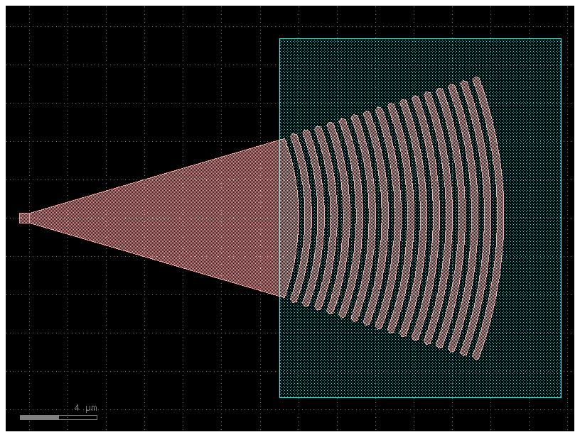
Simulate fiber-to-chip coupling in a compact 16-period generic-PDK elliptical grating coupler with gsim.fdtd on a 60 nm Yee grid. A tilted Gaussian beam illuminates the grating; a 0.5 µm straight waveguide gives the guided port o1 a uniform section for mode measurement. The grating pitch, taper, and beam position were tuned for coupling near 1.554 µm.
Requirements: gsim>=0.8.0 and GDSFactory+ cloud simulation access. To update an older project environment, run uv add "gsim>=0.8.0" "pdk-schema[sympy]~=0.3.0" from your project folder, then restart the notebook kernel.
Build the generic-PDK grating coupler
from math import cos, radians, sin

import gdsfactory as gf

from gsim import fdtd

FIBER_ANGLE_DEG = 15.0
FIBER_HEIGHT_UM = 1.05
BEAM_WAIST_UM = 5.0
TAPER_LENGTH_UM = 14.0
GRATING_DESIGN_WAVELENGTH_UM = 1.510
BEAM_OFFSET_UM = 4.5
Z_BOUNDS = (-1.0, 1.55)
pdk = gf.gpdk.PDK
pdk.activate()
component = gf.Component()
grating = component.add_ref(
    gf.components.grating_coupler_elliptical(
        fiber_angle=FIBER_ANGLE_DEG,
        n_periods=16,
        taper_length=TAPER_LENGTH_UM,
        wavelength=GRATING_DESIGN_WAVELENGTH_UM,
    )
)
straight = component.add_ref(gf.components.straight(length=0.5))
straight.connect("o2", grating.ports["o1"])
component.add_port("o1", port=straight.ports["o1"])
component.add_port("o2", port=grating.ports["o2"])
component
Place the fiber beam and flux monitor
The straight provides guided port o1; the grating provides vertical fiber port o2. Place the 15° Gaussian beam 4.5 µm toward the grating teeth from o2. A horizontal flux plane below the source measures net downward power entering the device region.
fiber_port = component.ports["o2"]
fiber_x_um, fiber_y_um = map(float, fiber_port.center)
beam_x_um = fiber_x_um + BEAM_OFFSET_UM
fiber_angle_rad = radians(FIBER_ANGLE_DEG)
beam_center_um = (beam_x_um, fiber_y_um, FIBER_HEIGHT_UM)
beam_size_um = (2 * BEAM_WAIST_UM, 2 * BEAM_WAIST_UM, 0.0)
fiber_direction = (-sin(fiber_angle_rad), 0.0, -cos(fiber_angle_rad))
simulation = fdtd.Simulation(pdk=pdk)
simulation.materials(background="sio2", overrides={"si": 3.47, "sio2": 1.443})
simulation.geometry(component, mesh_size_nm=500, geometry_tolerance_nm=20)
simulation.source = fdtd.GaussianBeamSource(
    center_um=beam_center_um,
    size_um=beam_size_um,
    aperture_normal="-z",
    propagation_direction=fiber_direction,
    e_polarization=(0.0, 1.0, 0.0),
    focal_point_um=(beam_x_um, fiber_y_um, 0.22),
    waist_radius_um=BEAM_WAIST_UM,
    refractive_index=1.443,
    wavelength_um=1.554,
    wavelength_span_um=0.1,
    num_wavelengths=101,
)
simulation.monitors.add_plane(
    name="src_down",
    center_um=(beam_x_um, fiber_y_um, 0.4),
    size_um=beam_size_um,
    normal="-z",
    flux=True,
)
simulation.domain(padding=0.5, z_bounds=Z_BOUNDS, pml_cells=16)
simulation.solver(cell_size_nm=60, energy_decay_fraction=1e-5, max_wall_seconds=3600)
Solver(cell_size_nm=60.0, max_timesteps=None, energy_decay_fraction=1e-05, max_wall_seconds=3600.0)
Inspect the 3D geometry
Preview the extruded layer stack, ports, and simulation domain before running.
Run and inspect coupling
Reuse a completed cloud job when the inputs match. The Gaussian beam is a free-space source, so the solver returns unnormalized guided-port power rather than a guided-port S-matrix column.
  fdtd-63dd1dd2  [####################] 100%  complete  elapsed 0m 00s


Extracting results.tar.gz...
Downloaded 2 files to /home/runner/work/simulation-templates/simulation-templates/docs/notebooks/sim-data-fdtd-63dd1dd2
import plotly.graph_objects as go

guided_power = result.port_outputs["o1"].modal_power
downward_flux = result.monitors["src_down"].flux

# Ignore wavelengths with less than 1% of the peak flux before dividing powers.
usable = result.valid & (downward_flux > 0.01 * downward_flux.max())
guided_fraction_percent = 100 * guided_power[usable] / downward_flux[usable]
figure = go.Figure()
figure.add_scatter(
    x=result.wavelength_um[usable],
    y=guided_fraction_percent,
    mode="lines",
    name="o1",
)
figure.update_layout(
    xaxis_title="Wavelength (µm)",
    yaxis_title="Guided fraction of net downward flux (%)",
)
figure
Reflected light crosses src_down upward, so the plotted net-flux fraction is higher than incident-normalized coupling. At 1.554 µm, a separate grating-free reference gives 31.0% guided power relative to the incoming beam for this 60 nm setup.