This notebook creates spatial wafer maps for ridge waveguides, following the same structure as notebook 5 for rib waveguides. The workflow is identical: query die JSONs by tag, group by wafer and width, and trigger the aggregation pipeline per group. Reusing the same analysis path for a different waveguide type is possible because the parameters were captured as tags rather than baked into separate folder structures.
Ridge waveguides are fully etched through the silicon layer. The deeper etch confines the optical mode more tightly, which is useful for compact bends, but it also brings more of the mode in contact with the sidewalls. Sidewall roughness from the lithography and etch process scatters light out of the mode, resulting in higher propagation loss than rib waveguides at the same width.
The spec limits here (1.5 to 6.5 dB/cm) are shifted higher than the rib limits (0.5 to 4.5 dB/cm) to reflect this expected difference. In a real process qualification you would derive these limits from historical data and product requirements.
Setup
import getpass
from pathlib import Path

import gfhub
from gfhub import nodes
from PIL import Image
from tqdm.auto import tqdm

client = gfhub.Client()
user = getpass.getuser()
print(f"Running as user: {user}")
Running as user: runner
Re-upload the wafer map function
The same spirals_wafer_map.py used for rib waveguides in notebook 5 is re-uploaded here. Calling add_function again is safe: it updates the existing definition if one with the same name already exists. Only the spec limits change, and those are passed as pipeline kwargs rather than baked into the function.
from spirals_wafer_map import main as spirals_wafer_map

func_def = gfhub.Function(
    spirals_wafer_map,
    dependencies={
        "json": "import json",
        "numpy": "import numpy as np",
        "matplotlib": [
            "import matplotlib.pyplot as plt",
            "import matplotlib.colors as mcolors",
        ],
    },
)
client.add_function(func_def, name="spirals_wafer_map")
print("spirals_wafer_map ready.")
spirals_wafer_map ready.
Creating the pipeline
The spec limits are 1.5 to 6.5 dB/cm, appropriate for ridge waveguides. The output_key is "propagation_loss", matching the field in the die analysis JSONs from notebook 4. Because the pipeline is registered server-side, running this for a new wafer lot requires only triggering it with the relevant file IDs, not re-deploying any code.
p = gfhub.Pipeline()

p.trigger = nodes.on_manual_trigger()
p.load_file = nodes.load()
p.load_tags = nodes.load_tags()
p += p.trigger >> p.load_file
p += p.trigger >> p.load_tags

p.find_common_tags = nodes.function(function="find_common_tags")
p += p.load_tags >> p.find_common_tags

p.aggregate = nodes.function(
    function="spirals_wafer_map",
    kwargs={
        "output_key": "propagation_loss",
        "min_output": 1.5,
        "max_output": 6.5,
    },
)
p += p.load_file >> p.aggregate

p.save = nodes.save()
p += p.aggregate >> p.save[0]
p += p.find_common_tags >> p.save[1]

confirmation = client.add_pipeline(name="ridge_wafer_analysis", schema=p)
print(f"Pipeline ready: {client.pipeline_url(confirmation['id'])}")
Pipeline ready: https://api.dev.gdsfactory.com/pipelines/019df3c4-2cd9-7e81-97ac-e15eec8d6260
Trigger per (wafer, width) group
We query the ridge propagation loss JSONs and group by wafer and width, giving one wafer map per width. Grouping by (wafer, width_nm) works because both were set as tags when the die analysis results were saved. Without tags, separating ridge results by width across a full wafer would require either a naming convention or a separate tracking file.
entries = client.query_files(
    name="propagation_loss_ridge_*.json",
    tags=["project:tutorial_spirals", user],
).groupby("wafer", "width_nm")

print(f"Found {len(entries)} (wafer, width) group(s)")

job_ids = []
for group_key, group in tqdm(entries.items()):
    print(f"  {group_key}: {len(group)} dies")
    input_ids = [f["id"] for f in group]
    triggered = client.trigger_pipeline("ridge_wafer_analysis", input_ids)
    job_ids.extend(triggered["job_ids"])

print(f"Triggered {len(job_ids)} wafer analysis job(s)")
Found 3 (wafer, width) group(s)


  0%|          | 0/3 [00:00<?, ?it/s]


  ('wafer:wafer_tutorial', 'width_nm:800'): 4 dies


  ('wafer:wafer_tutorial', 'width_nm:500'): 4 dies


  ('wafer:wafer_tutorial', 'width_nm:300'): 4 dies
Triggered 3 wafer analysis job(s)
jobs = client.wait_for_jobs(job_ids)
print(f"All jobs complete. Statuses: {set(j['status'] for j in jobs)}")
  0%|          | 0/3 [00:00<?, ?it/s]


All jobs complete. Statuses: {'success'}
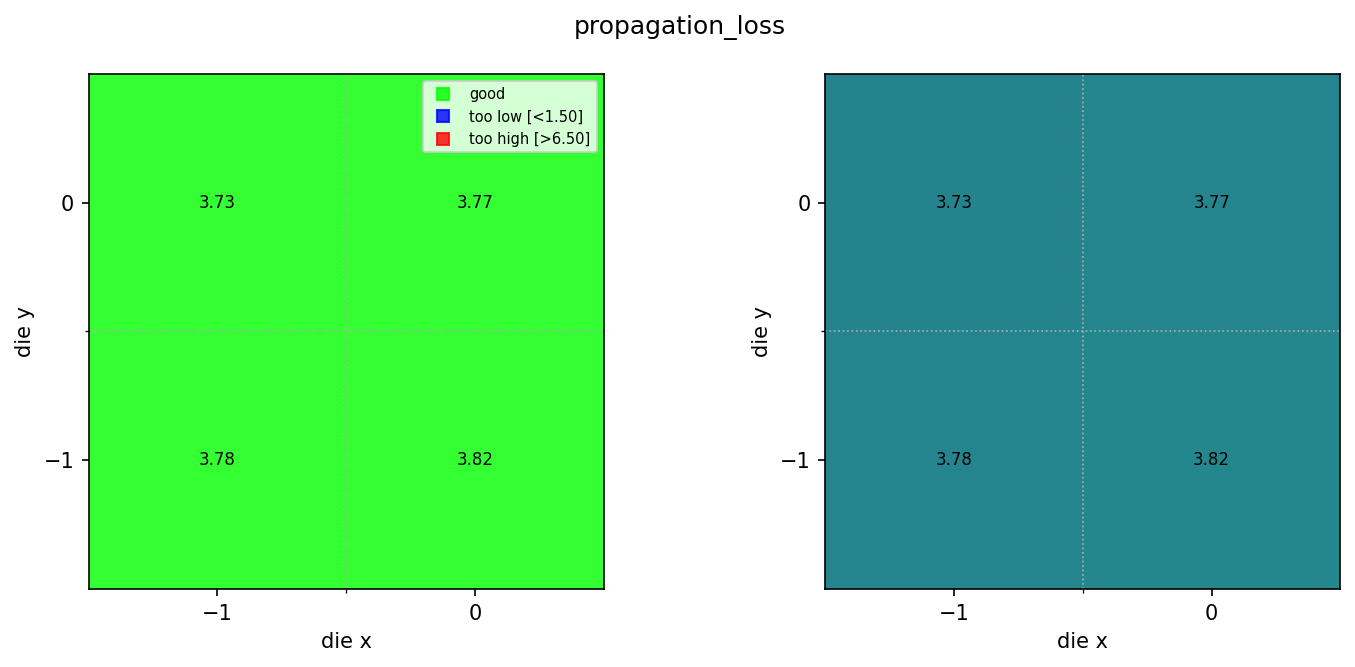
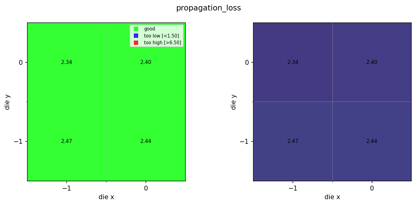
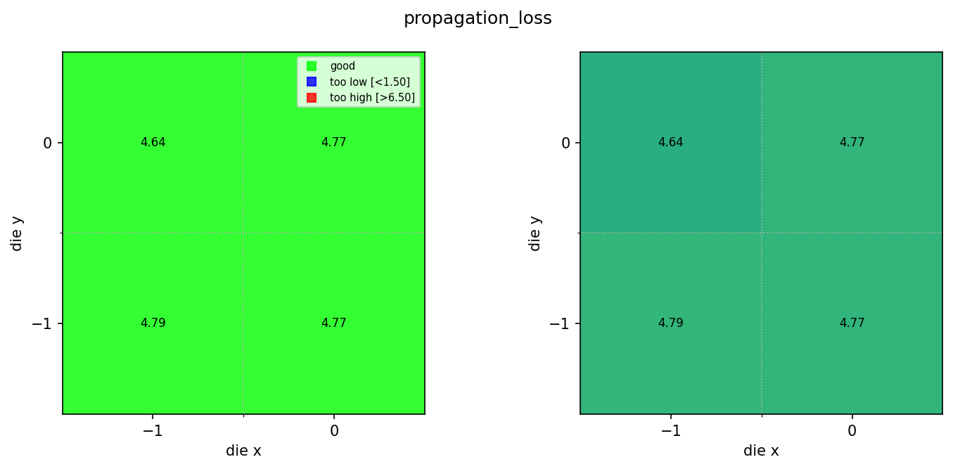
View the wafer maps
wafer_maps = client.query_files(
    name="wafer_map.png",
    tags=["project:tutorial_spirals", user, "waveguide_type:ridge"],
)
print(f"Found {len(wafer_maps)} ridge wafer maps")

for wm in wafer_maps:
    img = Image.open(client.download_file(wm["id"]))
    display(img)
Found 3 ridge wafer maps
Compare rib and ridge results
Now that both rib and ridge maps are available, you can query both sets of die JSONs and compare the mean propagation loss across waveguide types. A consistent offset between rib and ridge that matches the expected physics (higher loss for full etch) is a sign that the measurement is working correctly. Unexpected similarity could indicate a measurement artifact.
import json
import matplotlib.pyplot as plt
import numpy as np

rib_jsons = client.query_files(
    name="propagation_loss_rib_*.json", tags=["project:tutorial_spirals", user]
)
ridge_jsons = client.query_files(
    name="propagation_loss_ridge_*.json", tags=["project:tutorial_spirals", user]
)

def load_losses(entries):
    losses = {}
    for entry in entries:
        data = json.load(client.download_file(entry["id"]))
        w = data.get("width_nm")
        losses.setdefault(w, []).append(data["propagation_loss"])
    return {w: np.mean(v) for w, v in sorted(losses.items())}

rib_mean = load_losses(rib_jsons)
ridge_mean = load_losses(ridge_jsons)

widths = sorted(set(rib_mean) | set(ridge_mean))
x = np.arange(len(widths))

fig, ax = plt.subplots(figsize=(7, 4))
ax.bar(x - 0.2, [rib_mean.get(w, 0) for w in widths], 0.4, label="rib")
ax.bar(x + 0.2, [ridge_mean.get(w, 0) for w in widths], 0.4, label="ridge")
ax.set_xticks(x)
ax.set_xticklabels([f"{w} nm" for w in widths])
ax.set_xlabel("Width")
ax.set_ylabel("Mean propagation loss (dB/cm)")
ax.set_title("Rib vs. ridge propagation loss by width")
ax.legend()
ax.grid(True, alpha=0.3, axis="y")
plt.tight_layout()
plt.show()

print("Rib mean loss (dB/cm):", rib_mean)
print("Ridge mean loss (dB/cm):", ridge_mean)
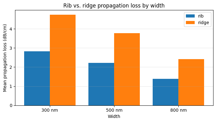
Rib mean loss (dB/cm): {300: np.float64(2.8192704853389143), 500: np.float64(2.2234896991906803), 800: np.float64(1.38929626150735)}
Ridge mean loss (dB/cm): {300: np.float64(4.7421945621871835), 500: np.float64(3.775385894736437), 800: np.float64(2.4128826986218597)}