Resistance measurement campaigns typically produce one file per device per die per wafer, with width and length encoded in the filename. That convention breaks as soon as a second person runs the same experiment and uses slightly different abbreviations, making it painful to collect all the width variants for a given die without a carefully maintained mapping spreadsheet.

Sheet resistance (measured in Ω/sq) is a fundamental parameter for any conductive thin film: doped silicon, metal traces, transparent conductors, and so on. It tells you how much resistance a square of the material presents, regardless of the square's size, and it feeds directly into device design for heaters, phase shifters, and contact resistance calculations.

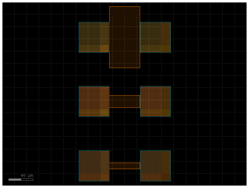
The standard way to extract it is to measure the resistance of rectangular test structures with different widths at a fixed length. Because resistance scales as R = Rs × L / W (where Rs is the sheet resistance, L is the length, and W is the width), a sweep of widths gives you multiple data points that you can fit to extract Rs.

This notebook generates a GDS layout containing three such test structures with widths of 10, 20, and 100 µm, all at the same length, and uploads it to DataLab.

Before you start, make sure your credentials are configured in ~/.gdsfactory/gdsfactoryplus.toml:

[tool.gdsfactoryplus.api]
key = "{your-api-key}"

[tool.gdsfactoryplus.hub]
host = "https://{organization}.hub.gdsfactory.com"

Setup¶

import getpass

import gdsfactory as gf
import gfhub
from gdsfactory.gpdk import PDK

PDK.activate()
client = gfhub.Client()
user = getpass.getuser()
print(f"Running as user: {user}")

Matplotlib is building the font cache; this may take a moment.


Running as user: runner

Creating the layout¶

gf.c.resistance_sheet generates a four-terminal test structure for a sheet of given width. We wrap it in a cell function so GDSFactory can cache it by parameter, then generate one instance per target width.

We use gf.grid to arrange the three structures in a column. Unlike gf.pack (which uses bin-packing to minimize space), gf.grid places cells in a regular row/column arrangement. For a small, ordered set of test structures this is the right choice: the regular layout makes it easy to navigate on a probe station.

@gf.cell
def resistance_sheet(width=10) -> gf.Component:
    return gf.c.resistance_sheet(width=width)


@gf.cell
def resistance() -> gf.Component:
    widths = (10, 20, 100)
    sweep = [resistance_sheet(width=width) for width in widths]
    # Stack the three structures in a single column
    return gf.grid(sweep, shape=(len(sweep), 1))


c = resistance()
c.write_gds("resistance.gds")
c.plot()

Upload the GDS¶

We upload the layout file tagged with project:tutorial_resistance and your username. These two tags will appear on every file in this tutorial series, so any query that includes both will return only files from your run of this specific project. Attaching the project tag here means the layout stays findable alongside its measurement data later, without needing a separate tracking spreadsheet.

uploaded = client.add_file("resistance.gds", tags=["project:tutorial_resistance", user])
print(f"Uploaded: {uploaded['original_name']} (id={uploaded['id']})")

Uploaded: resistance.gds (id=019df3b5-566e-72b0-b617-9a1420ad51ad)

What's next?¶

The layout is now in DataLab. The next notebook loads this GDS, simulates IV measurements for each test structure across a set of wafers and dies, and uploads all the measurement data with the appropriate provenance tags.