Each spectrum uploaded in the previous notebook spans a 100 nm wavelength range. For the propagation loss fit in notebook 4 we need a single scalar per device: the transmitted power at a specific wavelength. Reducing the spectrum to this one number is what the device analysis pipeline does. Running this reduction consistently across all files is exactly the kind of repetitive step that tends to happen differently each time someone runs it manually.
The target wavelength is 1550 nm, the centre of the C-band and the peak of the grating coupler response. Before reading the power at that wavelength, we apply a short rolling-window average to reduce measurement noise. The window is small enough that it does not bias the value, but it eliminates point-to-point spikes that can arise from laser power fluctuations or detector noise.
The pipeline is set up with both an auto-trigger and a manual trigger: - The auto-trigger fires on every new spectrum upload, so future measurements are processed immediately. - The manual trigger is used at the end of this notebook to backfill all the spectra already in DataLab.
Setup
import getpass
import json
from pathlib import Path

import gfhub
import matplotlib.pyplot as plt
import numpy as np
import pandas as pd
from gfhub import nodes
from PIL import Image
from tqdm.auto import tqdm

client = gfhub.Client()
user = getpass.getuser()
print(f"Running as user: {user}")
Running as user: runner
Load a sample spectrum
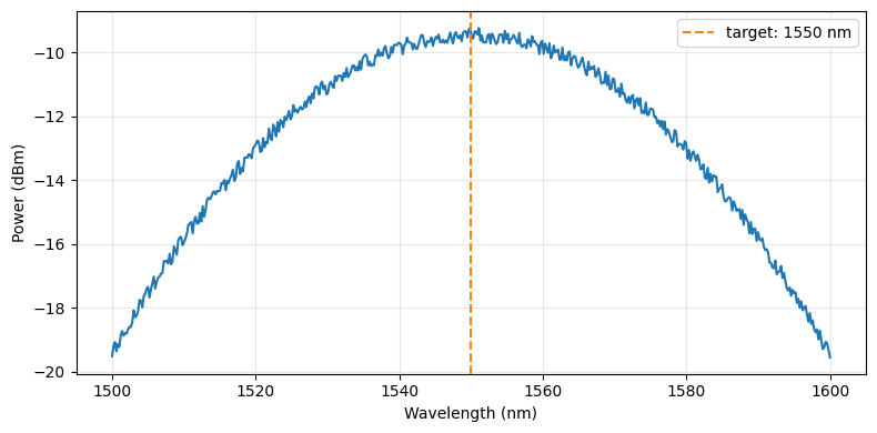
Before building the pipeline we load one spectrum interactively to verify the data format and confirm that the target wavelength falls within the sweep range.
sample_entry = client.query_files(
    tags=["project:tutorial_spirals", user, ".parquet", "waveguide_type:rib", "width_nm:500"]
).newest()

sample_path = Path("sample_spectrum.parquet")
client.download_file(sample_entry["id"], sample_path)
sample_df = pd.read_parquet(sample_path)
print(sample_df.head())

fig, ax = plt.subplots(figsize=(8, 4))
ax.plot(sample_df["wavelength"], 10 * np.log10(sample_df["output_power"] + 1e-12))
ax.axvline(1550, color="C1", linestyle="--", label="target: 1550 nm")
ax.set_xlabel("Wavelength (nm)")
ax.set_ylabel("Power (dBm)")
ax.legend()
ax.grid(True, alpha=0.3)
plt.tight_layout()
plt.show()
    wavelength  output_power
0  1500.000000      0.011199
1  1500.200401      0.012039
2  1500.400802      0.012390
3  1500.601202      0.011593
4  1500.801603      0.012227
Defining the device analysis function
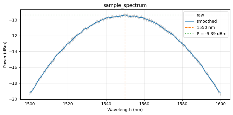
spiral_power_at_wavelength reads the spectrum Parquet file, smooths it with a rolling window, and extracts the power at target_nm. The window parameter sets how many wavelength points to average. With 500 points over 100 nm the step size is 0.2 nm, so window=11 averages about 2 nm, which is small compared to the grating coupler bandwidth of 100 nm.
The JSON output contains two power fields: power (linear, mW) and power_dBm (decibels). The die analysis in notebook 4 uses power_dBm for the linear regression, because loss in dB is linear in length.
def spiral_power_at_wavelength(
    path: Path,
    /,
    *,
    xname: str = "wavelength",
    yname: str = "output_power",
    target_nm: float = 1550.0,
    window: int = 11,
) -> tuple[Path, Path]:
    """Extract power at a target wavelength from a spiral spectrum.

    Args:
        path: Path to Parquet file with columns `xname` (nm) and `yname` (mW).
        xname: Column name for wavelength.
        yname: Column name for output power.
        target_nm: Wavelength at which to read the power, in nm.
        window: Rolling average window size (number of wavelength points).

    Returns:
        Tuple of (plot PNG path, results JSON path).
    """
    df = pd.read_parquet(path)
    wl = df[xname].values
    power = df[yname].values

    # Rolling average to reduce noise before sampling at the target wavelength
    power_smooth = (
        pd.Series(power).rolling(window=window, center=True, min_periods=1).mean().values
    )

    # Nearest-neighbour lookup at the target wavelength
    idx = int(np.argmin(np.abs(wl - target_nm)))
    power_at_target = float(power_smooth[idx])

    fig, ax = plt.subplots(figsize=(8, 4))
    ax.plot(wl, 10 * np.log10(power + 1e-12), color="C7", alpha=0.4, label="raw")
    ax.plot(wl, 10 * np.log10(power_smooth + 1e-12), color="C0", label="smoothed")
    ax.axvline(target_nm, color="C1", linestyle="--", label=f"{target_nm:.0f} nm")
    ax.axhline(
        10 * np.log10(power_at_target + 1e-12),
        color="C2", linestyle=":", alpha=0.8,
        label=f"P = {10*np.log10(power_at_target+1e-12):.2f} dBm",
    )
    ax.set_xlabel("Wavelength (nm)")
    ax.set_ylabel("Power (dBm)")
    ax.set_title(path.stem)
    ax.legend()
    ax.grid(True, alpha=0.3)
    plt.tight_layout()

    plot_path = path.with_name(path.stem + "_analysis.png")
    plt.savefig(plot_path, bbox_inches="tight", dpi=100)
    plt.close()

    results = {
        "power": power_at_target,
        "power_dBm": float(10 * np.log10(power_at_target + 1e-12)),
        "target_wavelength_nm": target_nm,
    }
    results_path = path.with_name(path.stem + "_analysis.json")
    results_path.write_text(json.dumps(results, indent=2))

    return plot_path, results_path
func_def = gfhub.Function(
    spiral_power_at_wavelength,
    dependencies={
        "json": "import json",
        "pandas[pyarrow]": "import pandas as pd",
        "numpy": "import numpy as np",
        "matplotlib": "import matplotlib.pyplot as plt",
    },
)
Testing locally
Before uploading the function we run it locally on the sample spectrum. For a tuple-return function, result["output"] is a list with one element per return value.
result = func_def.eval(sample_path)
plot_path, json_path = result["output"]
print(json_path.read_text())
Image.open(plot_path)
{
  "power": 0.11515376204821766,
  "power_dBm": -9.387218691584819,
  "target_wavelength_nm": 1550.0
}
spiral_power_at_wavelength uploaded.
Creating the pipeline
The pipeline has an auto-trigger and a manual trigger wired to the same load nodes. The auto-trigger means each new spectrum gets a device analysis result automatically. The function is registered server-side, so it runs consistently regardless of who uploaded the file. The manual trigger is used below to backfill existing files.
Because the function returns two files (plot and JSON), we use two separate save nodes. Both receive the original file's tags via load_tags >> save[1], which is how each output inherits the die, waveguide_type, width_nm, and length_um tags from the input spectrum.
p = gfhub.Pipeline()

p.auto_trigger = nodes.on_file_upload(tags=[".parquet", "project:tutorial_spirals", user])
p.manual_trigger = nodes.on_manual_trigger()
p.load_file = nodes.load()
p.load_tags = nodes.load_tags()

p += p.auto_trigger >> p.load_file
p += p.manual_trigger >> p.load_file
p += p.auto_trigger >> p.load_tags
p += p.manual_trigger >> p.load_tags

p.analysis = nodes.function(
    function="spiral_power_at_wavelength",
    kwargs={"xname": "wavelength", "yname": "output_power", "target_nm": 1550.0},
)
p += p.load_file >> p.analysis

p.save_plot = nodes.save()
p.save_json = nodes.save()
p += p.analysis[0] >> p.save_plot[0]
p += p.load_tags >> p.save_plot[1]
p += p.analysis[1] >> p.save_json[0]
p += p.load_tags >> p.save_json[1]

confirmation = client.add_pipeline(name="spiral_device_analysis", schema=p)
print(f"Pipeline ready: {client.pipeline_url(confirmation['id'])}")
Pipeline ready: https://api.dev.gdsfactory.com/pipelines/019df3b7-d66a-7262-93a7-7482d84c74e5
Run analysis on all existing spectra
We trigger the pipeline once per uploaded spectrum file. Each trigger creates one job, which runs the function and saves the plot and JSON.
spectra = client.query_files(tags=["project:tutorial_spirals", user, ".parquet", "waveguide_type"])
print(f"Found {len(spectra)} spectrum files")

job_ids = []
for spectrum in tqdm(spectra):
    triggered = client.trigger_pipeline("spiral_device_analysis", spectrum["id"])
    job_ids.extend(triggered["job_ids"])

print(f"Triggered {len(job_ids)} analysis jobs")
Found 144 spectrum files


  0%|          | 0/144 [00:00<?, ?it/s]


Triggered 144 analysis jobs
jobs = client.wait_for_jobs(job_ids)
print(f"All jobs complete. Statuses: {set(j['status'] for j in jobs)}")
  0%|          | 0/144 [00:00<?, ?it/s]


All jobs complete. Statuses: {'success'}
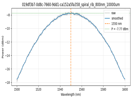
View a sample result
analysis_plots = client.query_files(name="*_analysis.png", tags=["project:tutorial_spirals", user])
print(f"Found {len(analysis_plots)} analysis plots")

if analysis_plots:
    img = Image.open(client.download_file(analysis_plots[0]["id"]))
    display(img.resize((530, 400)))
Found 287 analysis plots
analysis_jsons = client.query_files(name="*_analysis.json", tags=["project:tutorial_spirals", user])
print(f"Found {len(analysis_jsons)} analysis JSON files")

if analysis_jsons:
    data = json.load(client.download_file(analysis_jsons[0]["id"]))
    print(json.dumps(data, indent=2))
Found 287 analysis JSON files
{
  "power": 0.1671887724089616,
  "power_dBm": -7.767928910364885,
  "target_wavelength_nm": 1550.0
}
What's next?
Every device now has a power_dBm value at 1550 nm stored in DataLab. The next notebook groups these by (die, waveguide type, width) and fits the power vs. length relationship to extract the propagation loss in dB/cm for each group.