Aggregating device results at the die level is where filename-based workflows break down: you need to collect all width variants for each die, which means either parsing the width out of each filename or maintaining a separate device table. Because width and die coordinates were stored as tags at upload time, the groupby in this notebook just works.
Each device has a resistance R that depends on its dimensions: R = Rs × L / W. If you have measurements from multiple devices with different widths (or lengths) on the same die, you can rearrange to get Rs = R × W / L for each device individually, then average across devices on that die to reduce the per-device noise.
That is what this notebook does. We group the device-level JSON outputs (extracted resistance values) by die, and for each die we:
- Load the resistance, width, and length values from the JSON files and their tags
- Compute Rs = R × W / L for each device
- Report the mean and standard deviation as the die-level sheet resistance estimate
- Save a plot and a JSON summary back to DataLab tagged with the die's provenance
Setup
import getpass
import json
from pathlib import Path

import gfhub
import matplotlib.pyplot as plt
import numpy as np
from gfhub import nodes
from PIL import Image
from tqdm.auto import tqdm

client = gfhub.Client()
user = getpass.getuser()
print(f"Running as user: {user}")
Running as user: runner
Load a sample group to verify the data
Before building the pipeline function, we download the device analysis JSONs for one die and inspect the data. groupby("wafer", "die") returns a dictionary keyed by (wafer, die) tuples, where each value is the list of files belonging to that group. This works because wafer and die were set as structured tags at upload time, so there is no filename to parse and no separate device table to maintain.
gfhub.tags.into_string converts each tag object from the API response into a plain string of the form key:value or key, the same format the pipeline functions expect.
analysis_results = client.query_files(
    name="*_linear_fit.json", tags=["project:tutorial_resistance", user]
).groupby("wafer", "die")

# Pick one die to inspect
key = (wafer, die) = next(iter(analysis_results))
results = analysis_results[key]
print(f"Inspecting: wafer={wafer}, die={die}, {len(results)} devices")

paths = [
    client.download_file(r["id"], f"./download_{i}.json") for i, r in enumerate(results)
]
tags = [
    [gfhub.tags.into_string(t) for t in r["tags"].values()]
    for r in results
]

print("Sample tags:", tags[0])
Inspecting: wafer=wafer:wafer1, die=die:-1,-1, 6 devices


Sample tags: ['project:tutorial_resistance', 'wafer:wafer1', 'die:-1,-1', 'cell:resistance_sheet_W10', 'device:resistance_sheet_W10_0_52500', '.json', 'runner', 'length:50.0', 'width:10']
Defining the die-level analysis function
die_sheet_resistance receives a list of device JSON files and their corresponding tag lists. Width and length are stored as tags on each file (set when the measurement was uploaded in notebook 2), so we read them from file_tags rather than from inside the JSON itself.
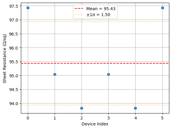
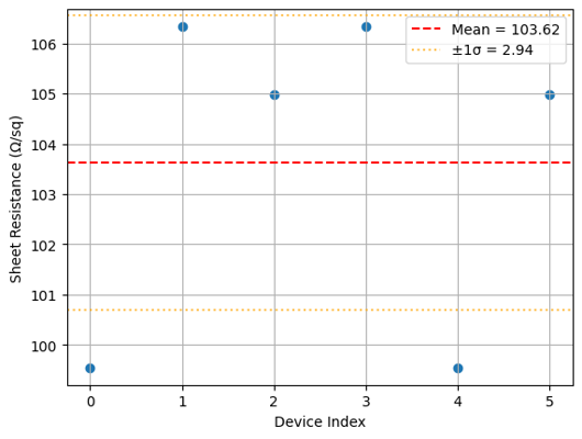
For each device with valid data, we compute R × W / L to recover the sheet resistance. The mean and standard deviation across all devices on the die give the die-level estimate. Open-circuit and short-circuit defects are excluded automatically because they produce extreme resistance values that would appear as outliers, though here we simply include all data and let the mean absorb the noise.
def die_sheet_resistance(
    files: list[Path],
    tags: list[list[str]],
    /,
    *,
    width_key: str = "width",
    length_key: str = "length",
) -> tuple[Path, Path]:
    """Aggregate device resistance measurements into a die-level sheet resistance estimate."""
    resistances, widths, lengths = [], [], []

    for file, file_tags in zip(files, tags, strict=False):
        data = json.loads(file.read_text())
        resistance = data.get("resistance")
        if resistance is None:
            continue

        # Width and length are stored as tags, not inside the JSON file
        width = next((float(t.split(":", 1)[1]) for t in file_tags if t.startswith(f"{width_key}:")), None)
        length = next((float(t.split(":", 1)[1]) for t in file_tags if t.startswith(f"{length_key}:")), None)

        if width is not None and length is not None:
            resistances.append(resistance)
            widths.append(width)
            lengths.append(length)

    if not resistances:
        msg = "No valid resistance measurements found"
        raise ValueError(msg)

    resistances = np.array(resistances)
    widths = np.array(widths)
    lengths = np.array(lengths)

    # Rs = R × W / L for each device
    rw_over_l = resistances * widths / lengths
    sheet_resistance = np.mean(rw_over_l)
    sheet_resistance_std = np.std(rw_over_l)

    # Plot the per-device sheet resistance estimates
    plt.scatter(range(len(rw_over_l)), rw_over_l)
    plt.axhline(sheet_resistance, color="r", linestyle="--", label=f"Mean = {sheet_resistance:.2f}")
    plt.axhline(sheet_resistance + sheet_resistance_std, color="orange", linestyle=":", alpha=0.7)
    plt.axhline(sheet_resistance - sheet_resistance_std, color="orange", linestyle=":", alpha=0.7, label=f"±1σ = {sheet_resistance_std:.2f}")
    plt.xlabel("Device Index")
    plt.ylabel("Sheet Resistance (Ω/sq)")
    plt.legend()
    plt.grid(True)
    plot_path = files[0].parent / "die_sheet_resistance.png"
    plt.savefig(plot_path, bbox_inches="tight", dpi=100)
    plt.close()

    # Extract die coordinates from tags for the wafer map in notebook 5
    die_x, die_y = None, None
    for tag in tags[0]:
        if tag.startswith("die:"):
            coords = tag.split(":", 1)[1]
            die_x, die_y = [int(c) for c in coords.split(",")]
            break

    results = {
        "die_x": die_x,
        "die_y": die_y,
        "sheet_resistance": float(sheet_resistance),
        "sheet_resistance_std": float(sheet_resistance_std),
        "num_devices": len(resistances),
    }
    results_path = files[0].parent / "die_sheet_resistance.json"
    results_path.write_text(json.dumps(results, indent=2))

    return plot_path, results_path
func_def = gfhub.Function(
    die_sheet_resistance,
    dependencies={
        "json": "import json",
        "numpy": "import numpy as np",
        "matplotlib": "import matplotlib.pyplot as plt",
    },
)
Testing locally
result = func_def.eval(paths, tags)
print(result)  # {"success": True, "output": ["/path/to/plot.png", "/path/to/results.json"]}

Image.open(result["output"][0])
{'success': True, 'output': (PosixPath('/home/runner/work/DataLab/DataLab/crates/sdk/examples/resistance/die_sheet_resistance.png'), PosixPath('/home/runner/work/DataLab/DataLab/crates/sdk/examples/resistance/die_sheet_resistance.json'))}
die_sheet_resistance uploaded.
Common tags
The outputs for each die should be tagged with the provenance shared by all devices on that die: the wafer, project, and username. Tags that vary between devices (cell, width, length, device name) should not appear on the aggregated output. find_common_tags handles this, exactly as in the cutback series.
def find_common_tags(tags: list[list[str]], /) -> list[str]:
    """Return only the tags that are identical across all input files."""
    common: dict[str, set] = {}
    for _tags in tags:
        for t in _tags:
            if ":" in t:
                key, value = t.split(":", 1)
            else:
                key, value = t, ""
            common.setdefault(key, set()).add(value)
    agreed = {k: next(iter(v)) for k, v in common.items() if len(v) == 1}
    return [k if not v else f"{k}:{v}" for k, v in agreed.items() if not k.startswith(".")]


client.add_function(find_common_tags)
print("find_common_tags uploaded.")
find_common_tags uploaded.
Creating the pipeline
p = gfhub.Pipeline()

p.trigger = nodes.on_manual_trigger()
p.load_file = nodes.load()
p.load_tags = nodes.load_tags()
p += p.trigger >> p.load_file
p += p.trigger >> p.load_tags

p.sheet_resistance = nodes.function(function="die_sheet_resistance")
p += p.load_file >> p.sheet_resistance[0]
p += p.load_tags >> p.sheet_resistance[1]

p.common_tags = nodes.function(function="find_common_tags")
p += p.load_tags >> p.common_tags

p.save_plot = nodes.save()
p.save_json = nodes.save()
p += p.sheet_resistance[0] >> p.save_plot[0]
p += p.common_tags >> p.save_plot[1]
p += p.sheet_resistance[1] >> p.save_json[0]
p += p.common_tags >> p.save_json[1]

confirmation = client.add_pipeline("die_sheet_resistance", p)
print(f"Pipeline ready: {client.pipeline_url(confirmation['id'])}")
Pipeline ready: https://api.dev.gdsfactory.com/pipelines/019df3b9-b753-7332-8a9d-222b4f92cd07
Trigger per die
We group all device JSON files by (wafer, die) and trigger the pipeline once per group. Each trigger passes all the device JSONs from one die, so the function can aggregate across devices. The grouping key comes directly from the tags attached at upload time, so the set of dies is discovered automatically rather than read from a hardcoded list.
analysis_results = client.query_files(
    name="*_linear_fit.json", tags=["project:tutorial_resistance", user]
).groupby("wafer", "die")

job_ids = []
for _key, files in tqdm(analysis_results.items()):
    input_ids = [f["id"] for f in files]
    triggered = client.trigger_pipeline("die_sheet_resistance", input_ids)
    job_ids.extend(triggered["job_ids"])

print(f"Triggered {len(job_ids)} die analysis jobs")
  0%|          | 0/8 [00:00<?, ?it/s]


Triggered 8 die analysis jobs
jobs = client.wait_for_jobs(job_ids)
print(f"All jobs complete. Statuses: {set(j['status'] for j in jobs)}")
  0%|          | 0/8 [00:00<?, ?it/s]


All jobs complete. Statuses: {'success'}
View a sample result
die_plots = client.query_files(
    name="die_sheet_resistance.png", tags=["project:tutorial_resistance", user]
)
print(f"Found {len(die_plots)} die analysis plots")

if die_plots:
    img = Image.open(client.download_file(die_plots[0]["id"]))
    display(img.resize((530, 400)))
Found 8 die analysis plots
What's next?
Each die now has a die_sheet_resistance.json in DataLab containing the sheet resistance estimate and the die coordinates. The next notebook loads all those JSON files, groups them by wafer, and builds the spatial wafer map.