Each spiral produces one swept-wavelength spectrum file. With two waveguide types, three widths, six lengths, and multiple dies per wafer, the number of files adds up quickly, and keeping the parameters straight is where filename conventions start to break down. Tags attached at upload time travel with each file so every downstream notebook can filter and group without relying on filename parsing.
In the previous notebook we generated the layout and uploaded the design manifest. Now we simulate swept-wavelength transmission spectra for each spiral device and upload them to DataLab.
The measurement setup sends a tunable laser through a grating coupler, along the spiral waveguide, and back out through a second grating coupler. The recorded transmission spectrum has two contributions:
- Grating coupler response: a Gaussian envelope centred at 1550 nm with a 1 dB bandwidth of ~100 nm. Two couplers are in the optical path, so their losses add.
- Waveguide propagation loss: the power decays exponentially with length. In dB, this is a linear term in length with slope equal to the propagation loss in dB/cm.
We model rib and ridge waveguides separately because their propagation losses differ: rib waveguides (partial etch) are lower loss than ridge waveguides (full etch). Within each type, narrower waveguides have higher loss because more of the optical mode interacts with the etched sidewalls.
We also set up an automatic plotting pipeline that fires on every new spectrum upload, so you get a preview plot for free without triggering anything manually.
Setup
import getpass
from contextlib import suppress
from pathlib import Path

import gfhub
import matplotlib.pyplot as plt
import numpy as np
import pandas as pd
from gfhub import nodes
from tqdm.auto import tqdm

np.random.seed(42)
client = gfhub.Client()
user = getpass.getuser()
print(f"Running as user: {user}")
Running as user: runner
Load the design manifest
We download the manifest uploaded in notebook 1 and use it to look up each device's width and length. Every simulated spectrum is tagged with width_nm and length_um so that downstream pipelines can group devices without re-reading the manifest.
manifest_entry = client.query_files(
    name="spirals_manifest.csv", tags=["project:tutorial_spirals", user]
).newest()
manifest = pd.read_csv(client.download_file(manifest_entry["id"]))
print(f"Manifest: {len(manifest)} devices")
manifest.head()
Manifest: 36 devices
| cell | waveguide_type | width_um | length_um | x | y | |
|---|---|---|---|---|---|---|
| 0 | cutback_rib_assembled_MFalse_W0p3_L0 | rib | 0.3 | 0 | 20150 | 60150 |
| 1 | cutback_rib_assembled_MTrue_W0p3_L25000 | rib | 0.3 | 25000 | 1039250 | 60150 |
| 2 | cutback_rib_assembled_MFalse_W0p3_L5000 | rib | 0.3 | 5000 | 20150 | 204150 |
| 3 | cutback_rib_assembled_MTrue_W0p3_L20000 | rib | 0.3 | 20000 | 1039250 | 204150 |
| 4 | cutback_rib_assembled_MFalse_W0p3_L10000 | rib | 0.3 | 10000 | 20150 | 348150 |
The transmission model
The gaussian_grating_coupler_response function returns the power through a single grating coupler as a function of wavelength. Two couplers are in the optical path (one in, one out), so we apply the response twice.
The waveguide attenuation follows Beer's law: each centimetre of waveguide attenuates the signal by loss_dB_per_cm dB. We add wafer-level variation (a random scalar applied to all devices on the same wafer) and device-level variation (a per-device scalar) to make the simulated data look like real measurements.
# Sweep parameters
wl_nm = np.linspace(1500.0, 1600.0, 500) # wavelength range, nm
wl0_nm = 1550.0 # grating coupler peak wavelength, nm
bw_1dB_nm = 100.0 # 1 dB bandwidth of grating coupler, nm
gc_loss_dB = 3.0 # per-coupler insertion loss, dB
# Propagation loss models (dB/cm) at widths [0.3, 0.5, 0.8] µm
# Rib waveguides are lower loss than ridge at the same width.
widths_um = np.array([0.3, 0.5, 0.8])
rib_losses_dBcm = np.array([3.0, 2.0, 1.5])
ridge_losses_dBcm = np.array([5.0, 3.5, 2.5])
rib_loss_model = np.polyfit(widths_um, rib_losses_dBcm, deg=1)
ridge_loss_model = np.polyfit(widths_um, ridge_losses_dBcm, deg=1)
# Variation parameters
wafer_variation = 0.20 # 20% wafer-to-wafer variation in peak power
device_variation = 0.05 # 5% device-to-device variation
noise_dB = 0.5 # peak-to-peak noise amplitude, dB
def gaussian_grating_coupler_response(
peak_power: float,
center_nm: float,
bw_1dB_nm: float,
wl_nm: np.ndarray,
) -> np.ndarray:
"""Return power through a Gaussian grating coupler vs. wavelength."""
sigma = bw_1dB_nm / (2 * np.sqrt(2 * np.log(10)))
return peak_power * np.exp(-0.5 * ((wl_nm - center_nm) / sigma) ** 2)
def simulate_spectrum(
wl_nm: np.ndarray,
width_um: float,
length_um: float,
waveguide_type: str,
wafer_factor: float,
) -> np.ndarray:
"""Simulate the transmission spectrum of a spiral waveguide device."""
# Peak power after both grating couplers (coupling loss only)
peak_power = 10 ** (-2 * gc_loss_dB / 10)
peak_power *= wafer_factor * (1 + device_variation * (2 * np.random.rand() - 1))
# Propagation loss through the spiral
loss_model = rib_loss_model if waveguide_type == "rib" else ridge_loss_model
loss_dB_per_cm = np.polyval(loss_model, width_um)
length_cm = length_um * 1e-4 # µm to cm
waveguide_attenuation = 10 ** (-loss_dB_per_cm * length_cm / 10)
# Full transmission: grating coupler envelope x waveguide attenuation x noise
envelope = gaussian_grating_coupler_response(peak_power, wl0_nm, bw_1dB_nm, wl_nm)
noise = 10 ** (noise_dB * np.random.rand(len(wl_nm)) / 10)
return envelope * waveguide_attenuation * noise
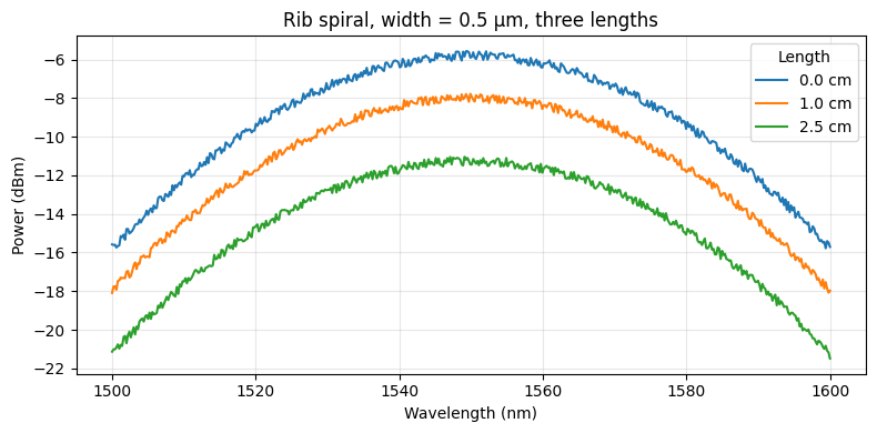
# Quick preview: rib, 0.5 µm, three different lengths
fig, ax = plt.subplots(figsize=(8, 4))
wafer_factor = 1.0
for length_um in [0, 10_000, 25_000]:
power = simulate_spectrum(wl_nm, 0.5, length_um, "rib", wafer_factor)
ax.plot(wl_nm, 10 * np.log10(power + 1e-12), label=f"{length_um/1e4:.1f} cm")
ax.set_xlabel("Wavelength (nm)")
ax.set_ylabel("Power (dBm)")
ax.set_title("Rib spiral, width = 0.5 µm, three lengths")
ax.legend(title="Length")
ax.grid(True, alpha=0.3)
plt.tight_layout()
plt.show()
Defining the plotting function
We want every measurement file we upload to automatically get a plot. To do this, we define a DataLab function that reads a Parquet spectrum and saves a plot of power vs. wavelength as a PNG. The function follows the standard convention: a positional-only Path input and a Path return value. Once uploaded, it can be wired into a pipeline that triggers on file upload.
def plot_spiral_spectrum(path: Path, /) -> Path:
    """Plot a swept-wavelength spectrum from a Parquet file and save as PNG."""
    df = pd.read_parquet(path)
    power_dBm = 10 * np.log10(df["output_power"].values + 1e-12)
    plt.figure(figsize=(8, 4))
    plt.plot(df["wavelength"].values, power_dBm)
    plt.xlabel("Wavelength (nm)")
    plt.ylabel("Power (dBm)")
    plt.title(path.stem)
    plt.xlim(df["wavelength"].min(), df["wavelength"].max())
    plt.grid(True)
    outpath = path.with_suffix(".png")
    plt.savefig(outpath, bbox_inches="tight")
    plt.close()
    return outpath


func_def = gfhub.Function(
    plot_spiral_spectrum,
    dependencies={
        "pandas[pyarrow]": "import pandas as pd",
        "numpy": "import numpy as np",
        "matplotlib": "import matplotlib.pyplot as plt",
    },
)
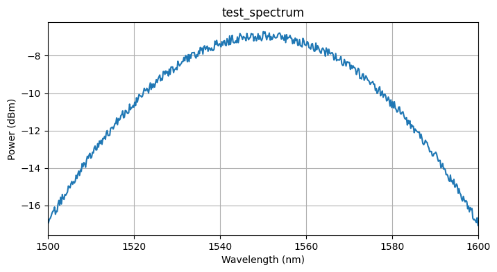
Testing locally
We test the function on a synthetic spectrum generated with the simulation model defined above. This runs the function in a sandboxed uv environment, the same way it will run on the server, so you can catch dependency or import errors before uploading.
# Generate a test spectrum using the simulation model
test_power = simulate_spectrum(wl_nm, 0.5, 5000, "rib", 1.0)
test_df = pd.DataFrame({"wavelength": wl_nm, "output_power": test_power})
test_path = Path("test_spectrum.parquet").resolve()
test_df.to_parquet(test_path)

result = func_def.eval(test_path)
print(result)  # {"success": True, "output": "/path/to/test_spectrum.png"}

from PIL import Image
Image.open(result["output"])
{'success': True, 'output': PosixPath('/home/runner/work/DataLab/DataLab/crates/sdk/examples/spirals/test_spectrum.png')}
plot_spiral_spectrum uploaded.
Creating the pipeline
A function on its own does nothing until it is wired into a pipeline. This pipeline triggers on any new .parquet file tagged with project:tutorial_spirals and your username. When it fires, it loads the file, runs plot_spiral_spectrum, and saves the resulting PNG back to DataLab with the same tags as the source file. The load_tags node carries the original file's tags through to the output, so the plot inherits the same provenance (die, waveguide_type, width_nm, length_um) as the spectrum it came from.
The manual trigger allows you to re-run the plot on any file after the fact, for example if you update the function and want to regenerate all plots.
p = gfhub.Pipeline()

p.auto_trigger = nodes.on_file_upload(tags=[".parquet", "project:tutorial_spirals", user])
p.manual_trigger = nodes.on_manual_trigger()
p.load = nodes.load()
p.load_tags = nodes.load_tags()
p.plot = nodes.function(function="plot_spiral_spectrum")
p.save = nodes.save()

p += p.auto_trigger >> p.load
p += p.manual_trigger >> p.load
p += p.auto_trigger >> p.load_tags
p += p.manual_trigger >> p.load_tags
p += p.load >> p.plot
p += p.plot >> p.save[0]
p += p.load_tags >> p.save[1]

confirmation = client.add_pipeline("plot_spiral_spectrum", p)
print(f"Pipeline ready: {client.pipeline_url(confirmation['id'])}")
Pipeline ready: https://api.dev.gdsfactory.com/pipelines/019df3b5-6eb7-75b0-a79a-a64e0c82dc3e
Clean up existing measurement files (optional)
existing = client.query_files(tags=["project:tutorial_spirals", user])
to_delete = [
    f for f in existing
    if f["original_name"] not in ("spirals.gds", "spirals_manifest.csv")
]
for f in tqdm(to_delete):
    with suppress(RuntimeError):
        client.delete_file(f["id"])
print(f"Deleted {len(to_delete)} file(s)")
  0%|          | 0/918 [00:00<?, ?it/s]


Deleted 918 file(s)
Generate and upload spectra
We simulate one spectrum per (wafer, die, device) combination. With four parameters per file (waveguide_type, width_nm, length_um, die), tags are more reliable than a filename convention: any downstream query uses query_files(tags=["waveguide_type:rib", "width_nm:500", "die:0,0"]) to get exactly the files needed for one propagation loss fit. The tags include waveguide_type, width_nm, and length_um so that notebooks 3 onwards can filter and group devices by these parameters without downloading the manifest again.
The wafer variation factor is drawn once per wafer to simulate a realistic spatial trend: all devices on the same wafer share the same baseline offset, then device-level variation is added on top.
for wafer in wafers:
    # One wafer-level variation factor, shared across all dies and devices
    wafer_factor = 1.0 + wafer_variation * (2 * np.random.rand() - 1)

    for die in tqdm(dies, desc=wafer):
        die_str = f"{die['x']},{die['y']}"

        for _, row in manifest.iterrows():
            width_um = row["width_um"]
            length_um = row["length_um"]
            waveguide_type = row["waveguide_type"]

            power = simulate_spectrum(
                wl_nm, width_um, length_um, waveguide_type, wafer_factor
            )
            df = pd.DataFrame({"wavelength": wl_nm, "output_power": power})

            client.add_file(
                df,
                tags=[
                    "project:tutorial_spirals",
                    user,
                    f"wafer:{wafer}",
                    f"die:{die_str}",
                    f"cell:{row['cell']}",
                    f"waveguide_type:{waveguide_type}",
                    f"width_nm:{int(width_um * 1000)}",
                    f"length_um:{int(length_um)}",
                ],
                filename=f"spiral_{waveguide_type}_{int(width_um*1000)}nm_{int(length_um)}um.parquet",
            )
wafer_tutorial: 0%| | 0/4 [00:00<?, ?it/s]
What's next?
All spectra are now in DataLab and the auto-plot pipeline is active. The next notebook defines the device analysis function, which reads each spectrum and extracts the transmitted power at the target wavelength (1550 nm). That single number per device is then used by notebook 4 to fit the propagation loss from the power vs. length relationship.