Uploading measurement data is where filename-based conventions tend to break down. A name like ring_r20um_g200nm_die_0_0.parquet works until someone renames a file, changes the separator, or forgets the gap value. Here we upload each spectrum with structured tags so the geometry and location are queryable directly, with no parsing required.
In the previous notebook we generated a chip layout with 9 ring resonator devices spanning three radii and three coupling gaps. Now we simulate swept-wavelength transmission spectra for each device and upload them to DataLab.
In this notebook we:
- Define the ring resonator physics model and the grating coupler envelope
- Simulate spectra with realistic noise and parameter variation
- Create an automatic plotting pipeline so every uploaded spectrum immediately gets a preview
- Upload the data for all devices across a set of wafers and dies
Setup
import getpass
from contextlib import suppress
from functools import cache
from itertools import product
from pathlib import Path

import gdsfactory as gf
import gfhub
import matplotlib.pyplot as plt
import numpy as np
import pandas as pd
from gdsfactory import gpdk
from gfhub import nodes
from tqdm.notebook import tqdm

gpdk.PDK.activate()
np.random.seed(42)
client = gfhub.Client()
user = getpass.getuser()
print(f"Running as user: {user}")
Running as user: runner
The ring resonator model
The ring function computes the all-pass filter transmission of a ring resonator as a function of wavelength. The physics are:
- The effective index
neffis linearly dispersive around the center wavelengthwl0, governed by the group indexng. - Round-trip loss is given by
lossin dB/m. - Coupling between bus and ring is set by
coupling, which determines the fraction of power transferred per pass.
The output is the normalised transmitted power (0 to 1) at each wavelength point. The resonances appear as dips in transmission — their spacing is the FSR.
# Simulation parameters
BW = 0.100       # 1 dB bandwidth of grating coupler, µm
P0 = 1.0         # peak power, mW
kappa2 = 0.1     # coupling coefficient
loss = 30e2      # waveguide loss, dB/m (= 30 dB/cm)
neff = 2.4       # effective index at wl0
ng = 4.0         # group index
wl0 = 1.550      # center wavelength, µm
gc_loss = 3      # grating coupler insertion loss, dB
wl = np.linspace(wl0 - 0.05, wl0 + 0.05, 500)  # wavelength sweep

# Noise parameters
noise = 0.1             # peak-to-peak noise amplitude, dB
ng_noise = 0.1          # group index variation
length_variability = 1  # ring length variation, µm
def ring(
    wl: np.ndarray,
    wl0: float,
    neff: float,
    ng: float,
    ring_length: float,
    coupling: float,
    loss: float,
) -> np.ndarray:
    """Return normalised all-pass transmission of a ring resonator.

    Args:
        wl: wavelength array, µm.
        wl0: reference wavelength for neff/ng, µm.
        neff: effective index at wl0.
        ng: group index (linear dispersion).
        ring_length: circumference, µm.
        coupling: power coupling coefficient (0–1).
        loss: propagation loss, dB/m.
    """
    transmission = 1 - coupling
    # Linear dispersion: neff shifts with wavelength
    neff_wl = neff + (wl0 - wl) * (ng - neff) / wl0
    # Round-trip field attenuation
    alpha = 10 ** (-loss * ring_length * 1e-6 / 20.0)
    phi = 2j * np.pi * neff_wl * ring_length / wl
    out = (np.sqrt(transmission) - alpha * np.exp(phi)) / (
        1 - np.sqrt(transmission) * alpha * np.exp(phi)
    )
    return abs(out) ** 2
def gaussian_grating_coupler_response(
    peak_power: float,
    center_wavelength: float,
    bandwidth_1dB: float,
    wavelength: np.ndarray,
) -> np.ndarray:
    """Return the Gaussian spectral envelope of a grating coupler."""
    sigma = bandwidth_1dB / (2 * np.sqrt(2 * np.log(10)))
    return peak_power * np.exp(-0.5 * ((wavelength - center_wavelength) / sigma) ** 2)
def noisy_spectrum(
    wl: np.ndarray,
    wl0: float,
    neff: float,
    ng: float,
    ring_length: float,
    coupling: float,
    loss: float,
    ideal_peak_power: float,
    bandwidth_1dB: float,
    noise_peak_to_peak_dB: float,
    noise_ng: float,
    ring_length_variability: float,
    grating_coupler_loss_dB: float,
) -> np.ndarray:
    """Return a simulated transmission spectrum with noise and fabrication variation."""
    # Attenuate peak power by grating coupler loss (two couplers in path)
    peak_power = ideal_peak_power * 10 ** (-2 * grating_coupler_loss_dB / 10)
    # Perturb group index and ring length to simulate process variation
    noisy_ng = ng + noise_ng * np.random.rand()
    noisy_length = ring_length + ring_length_variability * np.random.rand()
    envelope = gaussian_grating_coupler_response(peak_power, wl0, bandwidth_1dB, wl)
    spectrum = ring(wl, wl0, neff, noisy_ng, noisy_length, coupling, loss)
    noise_factor = 10 ** (noise_peak_to_peak_dB * np.random.rand(wl.shape[0]) / 10)
    return envelope * spectrum * noise_factor
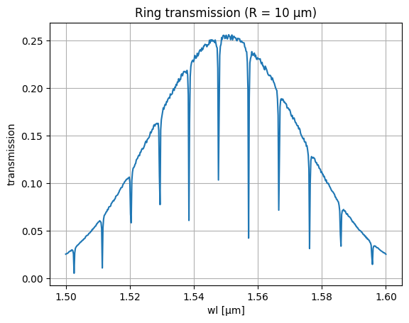
# Preview a single spectrum for R = 10 µm
L = 2 * np.pi * 10  # ring circumference, µm
thru = noisy_spectrum(wl, wl0, neff, ng, L, kappa2, loss, P0, BW, noise, ng_noise, length_variability, gc_loss)
plt.title("Ring transmission (R = 10 µm)")
plt.plot(wl, thru)
plt.grid(True)
plt.xlabel("wl [µm]")
plt.ylabel("transmission")
plt.show()
Auto-plotting pipeline
We define a plot_ring_spectrum function and wire it into a pipeline that fires automatically on every .parquet upload that carries the auto-plot:demo tag. The bulk uploads later in this notebook deliberately don't include that tag, so they don't trigger 36 plot jobs in CI. Instead we demonstrate the auto-trigger with a single demo upload at the end of the notebook.
In production you would tag every spectrum file with auto-plot:demo (or whatever filter you choose) so each upload fires its own preview job. That "one job per file" pattern is slower because each job pays container start-up cost, but it isolates failures: a single corrupt parquet doesn't bring down the others. Notebook 3 will contrast this with a batched pattern that processes many files in a single job.
def plot_ring_spectrum(path: Path, /) -> Path:
    """Plot ring transmission spectrum from a Parquet file and save as PNG."""
    df = pd.read_parquet(path)
    dB = 10 * np.log10(df.power.values)
    plt.plot(df.wl.values, dB)
    plt.xlabel("wl [µm]")
    plt.ylabel("power [dB]")
    plt.grid(visible=True)
    plt.title("ring spectrum")
    plt.xlim(df.wl.min(), df.wl.max())
    plt.ylim(None, 0)
    outpath = path.with_suffix(".png")
    plt.savefig(outpath, bbox_inches="tight")
    return outpath


func_def = gfhub.Function(
    plot_ring_spectrum,
    dependencies={
        "pandas[pyarrow]": "import pandas as pd",
        "numpy": "import numpy as np",
        "matplotlib": "import matplotlib.pyplot as plt",
    },
)
client.add_function(func_def)
print("plot_ring_spectrum uploaded.")
plot_ring_spectrum uploaded.
p = gfhub.Pipeline()

p.auto_trigger = nodes.on_file_upload(tags=[".parquet", "project:tutorial_rings", "auto-plot:demo", user])
p.manual_trigger = nodes.on_manual_trigger()
p.load = nodes.load()
p.load_tags = nodes.load_tags()
p.plot = nodes.function(function="plot_ring_spectrum")
p.save = nodes.save()

p += p.auto_trigger >> p.load
p += p.manual_trigger >> p.load
p += p.auto_trigger >> p.load_tags
p += p.manual_trigger >> p.load_tags
p += p.load >> p.plot
p += p.plot >> p.save[0]
p += p.load_tags >> p.save[1]

confirmation = client.add_pipeline("plot_ring_spectrum", p)
print(f"Pipeline ready: {client.pipeline_url(confirmation['id'])}")
Pipeline ready: https://api.dev.gdsfactory.com/pipelines/019df3b5-579b-7470-8b82-815542397054
Clean up existing files (optional)
existing_files = client.query_files(tags=["project:tutorial_rings", user])
to_delete = [f for f in existing_files if f["original_name"] != "rings.gds"]
for file in tqdm(to_delete):
    with suppress(RuntimeError):
        client.delete_file(file["id"])
0%| | 0/43 [00:00<?, ?it/s]
Load the layout
We import the GDS from notebook 1 to read the ring parameters stored on each cell. Each instance has inst.cell.info.radius (the ring radius in µm) which we use to compute the ring circumference and to tag the uploaded file.
Generate and upload spectra
We simulate one spectrum per combination of wafer, die, and device instance. The tags include radius_nm and ring_length_nm so downstream analysis can group by ring geometry without needing to re-read the GDS. These tags replace the filename convention: any later query can use query_files(tags=["radius_nm:20000"]) to get all 20 µm radius rings across every wafer, without glob patterns or a separate index file.
wafer_id = "wafer_tutorial"
wafers = [wafer_id]

dies = [
    {"x": x, "y": y}
    for y in range(-1, 1)
    for x in range(-1, 1)
]
for wafer, die in tqdm(list(product(wafers, dies))):
    die_str = f"{die['x']},{die['y']}"
    for inst in gds.insts:
        ring_length = 2 * np.pi * inst.cell.info.radius
        spectrum = noisy_spectrum(
            wl=wl,
            wl0=wl0, neff=neff, ng=ng,
            ring_length=ring_length,
            coupling=kappa2,
            loss=loss,
            ideal_peak_power=P0,
            bandwidth_1dB=BW,
            noise_peak_to_peak_dB=noise,
            noise_ng=ng_noise,
            ring_length_variability=length_variability,
            grating_coupler_loss_dB=gc_loss,
        )
        df = pd.DataFrame({"wl": wl, "power": spectrum})

        client.add_file(
            df,
            tags=[
                "project:tutorial_rings",
                user,
                f"wafer:{wafer}",
                f"die:{die_str}",
                f"cell:{inst.cell.name}",
                f"device:{inst.name}",
                f"radius_nm:{1000 * inst.cell.info.radius:.0f}",
                f"ring_length_nm:{1000 * ring_length:.0f}",
            ],
            filename=f"ring_{1000 * inst.cell.info.radius:.0f}.parquet",
        )
0%| | 0/4 [00:00<?, ?it/s]
Demonstrate the auto-trigger
The bulk upload above did not fire the plot_ring_spectrum pipeline because none of those files carry the auto-plot:demo tag. To show the auto-trigger working, we upload one extra spectrum tagged with auto-plot:demo. The pipeline fires immediately on the upload event and produces one preview PNG.
demo_radius = 10.0
demo_length = 2 * np.pi * demo_radius
demo_spectrum = noisy_spectrum(
    wl=wl, wl0=wl0, neff=neff, ng=ng,
    ring_length=demo_length,
    coupling=kappa2, loss=loss,
    ideal_peak_power=P0, bandwidth_1dB=BW,
    noise_peak_to_peak_dB=noise,
    noise_ng=ng_noise,
    ring_length_variability=length_variability,
    grating_coupler_loss_dB=gc_loss,
)
demo_df = pd.DataFrame({"wl": wl, "power": demo_spectrum})
demo_upload = client.add_file(
    demo_df,
    tags=[
        "project:tutorial_rings",
        user,
        "auto-plot:demo",
        f"wafer:{wafer_id}",
        f"radius_nm:{1000 * demo_radius:.0f}",
    ],
    filename="ring_demo_autoplot.parquet",
)
print(f"Demo file uploaded: {demo_upload}")
Demo file uploaded: {'id': '019df3b5-ac19-7a23-8176-61691ce96711', 'name': 'ring_demo_autoplot.parquet', 'original_name': 'ring_demo_autoplot.parquet', 'mime_type': 'application/octet-stream', 'status': 'Available'}
What's next?
The spectra are now in DataLab and the plotting pipeline is active. The next notebook defines the FSR analysis function, wraps it in a pipeline, and runs it on every uploaded spectrum to extract the resonance peak positions and FSR for each device.