Without an automated pipeline, fitting hundreds of IV curves typically means a manual batch script that someone has to remember to run after every measurement session. New files sit unanalysed until the next manual pass, and results files can easily end up scattered across local machines with no link back to their source data.
In the previous notebook we uploaded a synthetic IV curve for every device on every die. Now we need to extract a resistance value from each curve. Because V = R × I, the resistance is simply the slope of the voltage versus current line. We use scipy.stats.linregress to fit that slope and also get a quality metric (R² value) so we can flag noisy or defective measurements later.
In this notebook we:
- Define a
linear_fitfunction that takes a Parquet file and returns a plot and a JSON summary - Build a pipeline with both manual and automatic triggers, so any future upload of a matching file immediately gets analysed
- Run the pipeline on all the files already uploaded in notebook 2
Setup
import getpass
import json
from pathlib import Path

import gfhub
import matplotlib.pyplot as plt
import pandas as pd
from gfhub import nodes
from PIL import Image
from scipy import stats
from tqdm.auto import tqdm

client = gfhub.Client()
user = getpass.getuser()
print(f"Running as user: {user}")
Running as user: runner
Defining the analysis function
linear_fit takes a Parquet file and fits a straight line between two named columns. It is written as a general-purpose function (configurable column names, axis labels, and slope label) so it can be reused on any two-column linear dataset, not just IV curves.
The function returns two files: a PNG plot of the data and fit, and a JSON file with the extracted slope, intercept, R² value, and other fit statistics. These two outputs flow into separate save nodes in the pipeline.
def linear_fit(
    path: Path,
    /,
    *,
    xname: str,
    yname: str,
    slopename: str = "resistance",
    xlabel: str = "",
    ylabel: str = "",
) -> tuple[Path, Path]:
    """Fit a straight line between two columns in a Parquet file.

    Returns a plot PNG and a JSON with the fit parameters.
    """
    df = pd.read_parquet(path)
    x = df[xname].values
    y = df[yname].values

    slope, intercept, r_value, p_value, std_err = stats.linregress(x, y)

    _fig, ax = plt.subplots(figsize=(8, 6))
    ax.scatter(x, y, alpha=0.6, label="Data")
    ax.plot(
        x,
        slope * x + intercept,
        "r-",
        label=f"Fit: y = {slope:.3e}x + {intercept:.3e}",
    )
    ax.set_xlabel(xlabel or xname)
    ax.set_ylabel(ylabel or yname)
    ax.set_title(f"{slopename} = {slope:.3e} (R² = {r_value**2:.4f})")
    ax.legend()
    ax.grid(True)

    plot_path = path.with_name(path.stem + "_linear_fit.png")
    plt.savefig(plot_path, bbox_inches="tight", dpi=100)
    plt.close()

    results = {
        slopename: float(slope),
        "intercept": float(intercept),
        "r_squared": float(r_value**2),
        "p_value": float(p_value),
        "std_err": float(std_err),
    }
    results_path = path.with_name(path.stem + "_linear_fit.json")
    results_path.write_text(json.dumps(results, indent=2))

    return plot_path, results_path
func_def = gfhub.Function(
    linear_fit,
    dependencies={
        "matplotlib": "import matplotlib.pyplot as plt",
        "pandas[pyarrow]": "import pandas as pd",
        "scipy": "from scipy import stats",
        "json": "import json",
    },
)
Testing locally
We test the function on last_measurement.parquet saved by notebook 2. This runs the function in a sandboxed uv environment, the same way it will run on the server, so you can catch dependency or import errors before uploading.
path = Path("last_measurement.parquet").resolve()
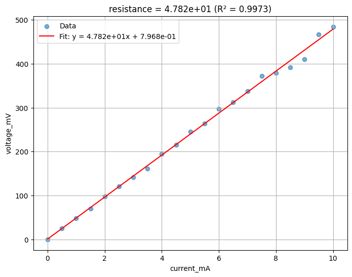
result = func_def.eval(path, xname="current_mA", yname="voltage_mV")
print(result)
Image.open(result["output"][0])
{'success': True, 'output': (PosixPath('/home/runner/work/DataLab/DataLab/crates/sdk/examples/resistance/last_measurement_linear_fit.png'), PosixPath('/home/runner/work/DataLab/DataLab/crates/sdk/examples/resistance/last_measurement_linear_fit.json'))}
linear_fit uploaded.
Creating the pipeline
This pipeline has both a manual trigger and an auto-trigger. The auto-trigger fires whenever a .parquet file with the right set of tags is uploaded, so any new measurement you upload will be automatically analysed without a manual batch step. Tags without explicit values (like "wafer", "die") match any file that has that tag regardless of value, which is how the trigger becomes general across all wafers and dies.
The pipeline loads the file, runs linear_fit with the IV column names, and saves the plot and JSON back to DataLab with the same tags as the source file.
p = gfhub.Pipeline()

# Auto-trigger on any matching .parquet upload; manual trigger for backfill
p.auto_trigger = nodes.on_file_upload(
    tags=[".parquet", user, "project:tutorial_resistance", "wafer", "die", "cell", "device", "length", "width"]
)
p.trigger = nodes.on_manual_trigger()

p.load_file = nodes.load()
p.load_tags = nodes.load_tags()
p += p.auto_trigger >> p.load_file
p += p.auto_trigger >> p.load_tags
p += p.trigger >> p.load_file
p += p.trigger >> p.load_tags

# Run the fit with IV column names and label the extracted slope as 'resistance'
p.fit = nodes.function(
    function="linear_fit",
    kwargs={"xname": "current_mA", "yname": "voltage_mV", "slopename": "resistance"},
)
p += p.load_file >> p.fit

# Save plot (output 0) and JSON (output 1), both tagged with the source file's tags
p.save_plot = nodes.save()
p.save_json = nodes.save()
p += p.fit[0] >> p.save_plot[0]
p += p.load_tags >> p.save_plot[1]
p += p.fit[1] >> p.save_json[0]
p += p.load_tags >> p.save_json[1]

pipeline_id = client.add_pipeline(name="iv_resistance_fit", schema=p)["id"]
print(f"Pipeline ready: {client.pipeline_url(pipeline_id)}")
Pipeline ready: https://api.dev.gdsfactory.com/pipelines/019df3b5-e90c-7401-97a1-72194c65947e
Running analysis on all existing files
The auto-trigger only fires on new uploads. Because we uploaded the measurement data in notebook 2 before this pipeline existed, we need to trigger it manually for all those files now.
device_files = client.query_files(
    tags=[".parquet", user, "project:tutorial_resistance", "wafer", "die", "cell", "device", "length", "width"]
)
print(f"Found {len(device_files)} device files")

job_ids = []

for device_file in tqdm(device_files):
    triggered = client.trigger_pipeline("iv_resistance_fit", device_file["id"])
    job_ids.extend(triggered["job_ids"])

print(f"Triggered {len(job_ids)} analysis jobs")
Found 24 device files


  0%|          | 0/24 [00:00<?, ?it/s]


Triggered 24 analysis jobs
jobs = client.wait_for_jobs(job_ids)
print(f"All jobs complete. Statuses: {set(j['status'] for j in jobs)}")
  0%|          | 0/24 [00:00<?, ?it/s]


All jobs complete. Statuses: {'success'}
Viewing a sample result
analysis_plots = client.query_files(
    name="*_linear_fit.png", tags=["project:tutorial_resistance", user]
)
print(f"Found {len(analysis_plots)} analysis plots")

if analysis_plots:
    img = Image.open(client.download_file(analysis_plots[0]["id"]))
    display(img.resize((530, 400)))
Found 48 analysis plots
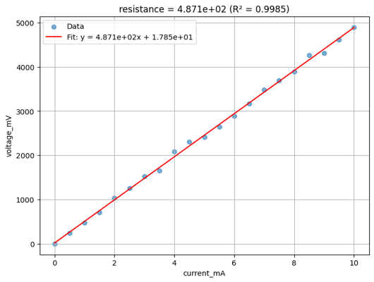
analysis_results = client.query_files(
    name="*_linear_fit.json", tags=["project:tutorial_resistance", user]
)
print(f"Found {len(analysis_results)} analysis result files")

if analysis_results:
    result_data = json.load(client.download_file(analysis_results[0]["id"]))
    print(json.dumps(result_data, indent=2))
Found 48 analysis result files
{
  "resistance": 487.14466509537715,
  "intercept": 17.84820114102513,
  "r_squared": 0.998520988114899,
  "p_value": 2.35436108337598e-28,
  "std_err": 4.301187582873236
}
What's next?
Each device now has a JSON file with its extracted resistance, stored in DataLab with the same provenance tags as the original measurement. The next notebook groups these JSON files by die and extracts the sheet resistance for each die using the R × W / L relationship across the three device widths.