Notebook 3 produced one combined FSR table for the whole wafer — one row per device, each row carrying the device's tags. Here we read that single file and roll it up into a per-(die, radius) summary so the wafer map in notebook 5 has something to plot.
The key subtlety is that rings of different radii have different FSRs (larger radius → longer circumference → smaller FSR), so averaging FSR across all radii on a die would be meaningless. We group rows by both die and radius_nm (read from each row's tags) and compute a mean FSR per group.
This notebook deliberately uses a different shape from notebook 3: rather than list[Path] per group, it consumes the single combined JSON and groups internally. That asymmetry illustrates the third granularity on the per-file ↔ batched spectrum: read once, fan out the grouping in Python.
Setup
import getpass
import json
from pathlib import Path

import gfhub
import matplotlib.pyplot as plt
import numpy as np
from gfhub import nodes
from PIL import Image

client = gfhub.Client()
user = getpass.getuser()
print(f"Running as user: {user}")
Running as user: runner
Load sample data
Download the combined FSR results JSON produced by notebook 3 so we can test the aggregation function locally before wiring it into a pipeline.
combined_entries = client.query_files(
    name="combined_fsr_results.json",
    tags=[user, "project:tutorial_rings"],
)
sample_combined_id = combined_entries.newest()["id"]

sample_path = Path("sample_combined.json").resolve()
client.download_file(sample_combined_id, sample_path)
sample_data = json.loads(sample_path.read_text())
print(f"Sample combined.json has {len(sample_data['rows'])} device rows")
print("First row tags:", sample_data["rows"][0]["tags"])
Sample combined.json has 36 device rows
First row tags: ['project:tutorial_rings', 'runner', 'wafer:wafer_tutorial', 'die:0,0', 'cell:RingDouble-5-0.2-', 'device:RingDouble-5-0.2-_331480_1044771', 'radius_nm:5000', 'ring_length_nm:31416']
Defining the aggregation function
fsr_wafer_aggregation reads the combined JSON, parses each row's tag list to extract die and radius_nm, groups the rows by (die_x, die_y, radius_nm), and emits a die_radius_table.json plus a summary scatter plot.
Note the shape change: input is a single Path (the combined JSON), not list[Path]. The grouping that notebook 3 would have done by triggering one call per group instead happens here in pure Python over a single in-memory list. That keeps the pipeline at one job per wafer instead of one per (die, radius) group.
def fsr_wafer_aggregation(combined: Path, /) -> tuple[Path, Path]:
"""Group device-level FSR rows by (die, radius_nm) and emit a wafer table.
Returns:
(summary_plot.png, die_radius_table.json)
"""
data = json.loads(combined.read_text())
rows_in = data.get("rows", [])
groups: dict[tuple[int, int, int], list[float]] = {}
for row in rows_in:
tag_dict = {}
for t in row["tags"]:
if ":" in t:
k, v = t.split(":", 1)
tag_dict[k] = v
if "die" not in tag_dict or "radius_nm" not in tag_dict:
continue
try:
die_x, die_y = (int(c) for c in tag_dict["die"].split(","))
radius_nm = int(tag_dict["radius_nm"])
except ValueError:
continue
if row.get("fsr_mean_um") is None:
continue
groups.setdefault((die_x, die_y, radius_nm), []).append(1000 * row["fsr_mean_um"])
table_rows = []
for (die_x, die_y, radius_nm), values in sorted(groups.items()):
arr = np.array(values)
table_rows.append({
"die_x": die_x,
"die_y": die_y,
"radius_nm": radius_nm,
"mean": float(arr.mean()),
"std": float(arr.std()),
"num_devices": int(arr.size),
})
out_dir = combined.parent
table_path = out_dir / "die_radius_table.json"
table_path.write_text(json.dumps({"rows": table_rows}, indent=2))
radii = sorted({r["radius_nm"] for r in table_rows})
fig, ax = plt.subplots(figsize=(8, 5))
for radius in radii:
means = [r["mean"] for r in table_rows if r["radius_nm"] == radius]
ax.scatter([radius] * len(means), means, alpha=0.7, label=f"R={radius} nm")
ax.set_xlabel("ring radius (nm)")
ax.set_ylabel("mean FSR (nm)")
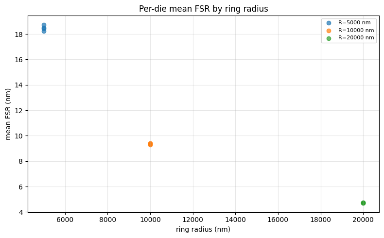
ax.set_title("Per-die mean FSR by ring radius")
ax.grid(True, alpha=0.3)
ax.legend(fontsize=8, loc="best")
plt.tight_layout()
plot_path = out_dir / "die_radius_summary.png"
plt.savefig(plot_path, bbox_inches="tight", dpi=100)
plt.close()
return plot_path, table_path
func_def = gfhub.Function(
    func=fsr_wafer_aggregation,
    dependencies={
        "json": "import json",
        "numpy": "import numpy as np",
        "matplotlib": "import matplotlib.pyplot as plt",
    },
)
result = func_def.eval(sample_path)
plot_path, table_path = result["output"]
table = json.loads(Path(table_path).read_text())
print(f"{len(table['rows'])} (die, radius) rows")
print(json.dumps(table["rows"][:3], indent=2))
Image.open(plot_path)
12 (die, radius) rows
[
  {
    "die_x": -1,
    "die_y": -1,
    "radius_nm": 5000,
    "mean": 18.420173680694745,
    "std": 0.33064445346063576,
    "num_devices": 3
  },
  {
    "die_x": -1,
    "die_y": -1,
    "radius_nm": 10000,
    "mean": 9.320121724931349,
    "std": 0.04728155068249648,
    "num_devices": 3
  },
  {
    "die_x": -1,
    "die_y": -1,
    "radius_nm": 20000,
    "mean": 4.736515637791875,
    "std": 0.00946199289531016,
    "num_devices": 3
  }
]
fsr_wafer_aggregation uploaded.
Creating the pipeline
The pipeline takes a single combined_fsr_results.json file ID, runs fsr_wafer_aggregation on it, and saves both outputs (summary plot and per-(die, radius) table JSON) tagged with the input file's provenance. One job per wafer.
p = gfhub.Pipeline()

p.trigger = nodes.on_manual_trigger()
p.load_file = nodes.load()
p.load_tags = nodes.load_tags()
p += p.trigger >> p.load_file
p += p.trigger >> p.load_tags

p.aggregate = nodes.function(function="fsr_wafer_aggregation")
p += p.load_file >> p.aggregate

p.save_plot = nodes.save()
p.save_table = nodes.save()
p += p.aggregate[0] >> p.save_plot[0]
p += p.load_tags >> p.save_plot[1]
p += p.aggregate[1] >> p.save_table[0]
p += p.load_tags >> p.save_table[1]

confirmation = client.add_pipeline(name="die_fsr_aggregation", schema=p)
print(f"Pipeline ready: {client.pipeline_url(confirmation['id'])}")
Pipeline ready: https://api.dev.gdsfactory.com/pipelines/019df3b6-51fd-7631-a57f-90aeebd81724
Trigger the aggregation
Query the combined results file from notebook 3 and trigger the aggregation pipeline once per wafer.
combined_files = client.query_files(
    name="combined_fsr_results.json",
    tags=["project:tutorial_rings", user],
)
print(f"Found {len(combined_files)} combined result file(s)")

job_ids = []
for combined in combined_files:
    triggered = client.trigger_pipeline("die_fsr_aggregation", combined["id"])
    job_ids.extend(triggered["job_ids"])

print(f"Triggered {len(job_ids)} aggregation job(s)")
Found 1 combined result file(s)
Triggered 1 aggregation job(s)
jobs = client.wait_for_jobs(job_ids)
print(f"All jobs complete. Statuses: {set(j['status'] for j in jobs)}")
  0%|          | 0/1 [00:00<?, ?it/s]


All jobs complete. Statuses: {'success'}
View the summary
The summary plot shows the per-die mean FSR for each ring radius — clusters of points at the same x-position represent multiple dies on the wafer.
summaries = client.query_files(
    name="die_radius_summary.png",
    tags=["project:tutorial_rings", user],
)
print(f"Found {len(summaries)} summary plot(s)")

if summaries:
    img = Image.open(client.download_file(summaries[-1]["id"]))
    display(img)
Found 1 summary plot(s)

What's next?
The wafer now has a single die_radius_table.json with one row per (die_x, die_y, radius_nm) — exactly the input the next notebook will read to render the wafer map.