With hundreds of spectra uploaded across multiple dies and wafers, running FSR extraction manually would mean either a long batch script or remembering to rerun it whenever new data arrives. Here we define the analysis as a pipeline function and trigger it once.
Each ring transmission spectrum contains a series of resonance dips. The spacing between consecutive dips is the Free Spectral Range (FSR), which is related to ring geometry by:
FSR = λ² / (ng × L)
where λ is the center wavelength, ng is the group index, and L is the ring circumference.
This notebook demonstrates the batched counterpart to notebook 2's per-file auto-trigger: instead of one job per spectrum, we process every spectrum in a single job. That trades the per-file pattern's failure isolation (one bad file fails one job, others survive) for raw throughput — a single batched call has constant overhead instead of paying container startup once per file. For tutorial-scale workloads (and CI), batching is the right default; for messy production data where individual files may be corrupt, the per-file pattern from notebook 2 is safer.
Setup
import getpass
import json
from pathlib import Path

import gfhub
import matplotlib.pyplot as plt
import numpy as np
import pandas as pd
from gfhub import nodes
from PIL import Image
from scipy.signal import find_peaks
from tqdm.auto import tqdm

client = gfhub.Client()
user = getpass.getuser()
print(f"Running as user: {user}")
Running as user: runner
Load a sample spectrum
Before building the pipeline, we load one spectrum interactively to understand the data structure and check that the peak finder works correctly.
upload_id = client.query_files(
    name="ring_5000.parquet", tags=["project:tutorial_rings", user, "die:0,0"]
).newest()["id"]

sample_path = Path("sample_df.parquet").resolve()
sample_df = pd.read_parquet(client.download_file(upload_id, sample_path))
print(sample_df.head())
         wl     power
0  1.500000  0.025101
1  1.500200  0.026039
2  1.500401  0.026381
3  1.500601  0.026731
4  1.500802  0.027024
Defining the batched FSR analysis function
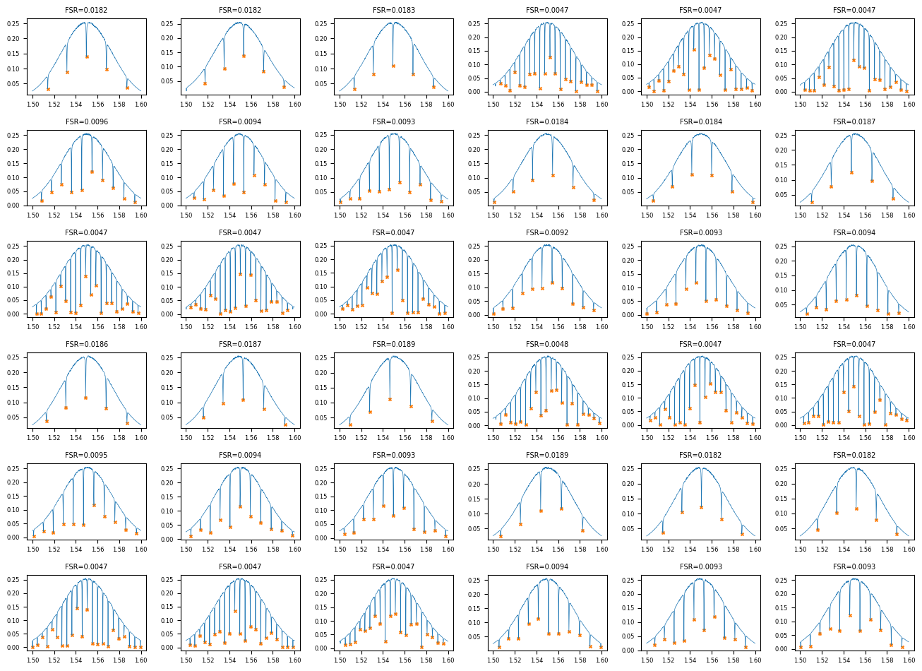
ring_fsr_batch accepts a list of input files and their tag lists, runs peak finding on each spectrum, and emits two outputs: a combined JSON with one row per input file (carrying the file's tags so notebook 4 can group on them) and a small grid PNG showing every spectrum at a glance.
The peak-finding logic is identical to the per-file form — scipy.signal.find_peaks on the negated power, with a prominence floor to reject noise. What's new is the loop and the JSON-as-table output shape. Notebook 4 will read this combined JSON and group by (die, radius_nm) internally, so we don't need a separate per-device JSON per file the way the previous version of this tutorial did.
def ring_fsr_batch(
    files: list[Path],
    tags: list[list[str]],
    /,
    *,
    xname: str = "wl",
    yname: str = "power",
    peaks_prominence: float = 0.01,
) -> tuple[Path, Path]:
    """Run FSR analysis on many spectra in one job.

    Returns:
        (summary_grid.png, combined_results.json)
    """
    rows = []
    n = len(files)
    cols = int(np.ceil(np.sqrt(n)))
    rows_grid = int(np.ceil(n / cols))
    fig, axes = plt.subplots(rows_grid, cols, figsize=(2.2 * cols, 1.6 * rows_grid))
    axes = np.atleast_1d(axes).ravel()

    for i, (path, file_tags) in enumerate(zip(files, tags)):
        df = pd.read_parquet(path)
        wavelength = df[xname].values
        power = df[yname].values
        peaks, _ = find_peaks(-power, prominence=peaks_prominence)

        if len(peaks) < 2:
            fsr_mean, fsr_std = None, None
            peak_wls = []
        else:
            peak_wls = wavelength[peaks].tolist()
            fsr_values = np.diff(peak_wls)
            fsr_mean = float(np.mean(fsr_values))
            fsr_std = float(np.std(fsr_values))

        rows.append({
            "tags": list(file_tags),
            "fsr_mean_um": fsr_mean,
            "fsr_std_um": fsr_std,
            "num_peaks": int(len(peaks)),
            "peak_wavelengths_um": [float(w) for w in peak_wls],
        })

        ax = axes[i]
        ax.plot(wavelength, power, lw=0.5, color="C0")
        if len(peaks) > 0:
            ax.scatter(wavelength[peaks], power[peaks], s=8, color="C1", marker="x")
        ax.set_title(f"FSR={fsr_mean:.4f}" if fsr_mean is not None else "no peaks", fontsize=7)
        ax.tick_params(labelsize=6)

    for j in range(n, len(axes)):
        axes[j].set_visible(False)

    plt.tight_layout()
    plot_path = files[0].parent / "fsr_summary_grid.png"
    plt.savefig(plot_path, bbox_inches="tight", dpi=100)
    plt.close()

    results_path = files[0].parent / "combined_fsr_results.json"
    results_path.write_text(json.dumps({"rows": rows}, indent=2))

    return plot_path, results_path
func_def = gfhub.Function(
    func=ring_fsr_batch,
    dependencies={
        "json": "import json",
        "numpy": "import numpy as np",
        "scipy": "from scipy.signal import find_peaks",
        "pandas[pyarrow]": "import pandas as pd",
        "matplotlib": "import matplotlib.pyplot as plt",
    },
)
Testing locally
For a tuple-return function, result["output"] is a list with one element per return value.
sample_tags = [
    "project:tutorial_rings", user, "wafer:wafer_tutorial",
    "die:0,0", "radius_nm:5000",
]
result = func_def.eval([sample_path], [sample_tags])
plot_path, json_path = result["output"]
print(json.dumps(json.loads(Path(json_path).read_text())["rows"][0], indent=2))
Image.open(plot_path)
{
  "tags": [
    "project:tutorial_rings",
    "runner",
    "wafer:wafer_tutorial",
    "die:0,0",
    "radius_nm:5000"
  ],
  "fsr_mean_um": 0.018236472945891813,
  "fsr_std_um": 0.0005109237989571347,
  "num_peaks": 5,
  "peak_wavelengths_um": [
    1.5142284569138276,
    1.5318637274549098,
    1.5498997995991985,
    1.5681362725450902,
    1.5871743486973948
  ]
}

client.add_function(func_def)
print("ring_fsr_batch uploaded.")


def find_common_tags(tags: list[list[str]], /) -> list[str]:
    """Return only the tags that are identical across all input files."""
    common: dict[str, set] = {}
    for _tags in tags:
        for t in _tags:
            if ":" in t:
                key, value = t.split(":", 1)
            else:
                key, value = t, ""
            common.setdefault(key, set()).add(value)
    agreed = {k: next(iter(v)) for k, v in common.items() if len(v) == 1}
    return [k if not v else f"{k}:{v}" for k, v in agreed.items() if not k.startswith(".")]


client.add_function(find_common_tags)
print("find_common_tags uploaded.")
ring_fsr_batch uploaded.
find_common_tags uploaded.
Creating the FSR analysis pipeline
This pipeline has a single manual trigger that accepts a list of file IDs. It loads all the files at once, runs ring_fsr_batch on the full list, and saves the two outputs (summary grid PNG and combined results JSON) tagged with the common provenance of the inputs (project, user, wafer). With one batched call instead of one call per file, the wafer's worth of analysis is one job rather than 36.
p = gfhub.Pipeline()

p.trigger = nodes.on_manual_trigger()
p.load_files = nodes.load()
p.load_tags = nodes.load_tags()
p += p.trigger >> p.load_files
p += p.trigger >> p.load_tags

p.fsr_batch = nodes.function(
    function="ring_fsr_batch",
    kwargs={"xname": "wl", "yname": "power", "peaks_prominence": 0.01},
)
p += p.load_files >> p.fsr_batch[0]
p += p.load_tags >> p.fsr_batch[1]

p.common_tags = nodes.function(function="find_common_tags")
p += p.load_tags >> p.common_tags

p.save_plot = nodes.save()
p.save_json = nodes.save()
p += p.fsr_batch[0] >> p.save_plot[0]
p += p.common_tags >> p.save_plot[1]
p += p.fsr_batch[1] >> p.save_json[0]
p += p.common_tags >> p.save_json[1]

confirmation = client.add_pipeline(name="rings_fsr_analysis", schema=p)
print(f"Pipeline ready: {client.pipeline_url(confirmation['id'])}")
Pipeline ready: https://api.dev.gdsfactory.com/pipelines/019df3b5-d2c0-7631-bdff-3ec6f6571a84
Trigger the batched analysis
One trigger_pipeline call with the list of all device file IDs starts a single job that processes every spectrum. The device tag filter excludes the auto-plot demo file from notebook 2 — that one had no device tag.
device_files = client.query_files(tags=["project:tutorial_rings", user, ".parquet", "device"])
print(f"Found {len(device_files)} device files")

input_ids = [f["id"] for f in device_files]
triggered = client.trigger_pipeline("rings_fsr_analysis", input_ids)
job_ids = triggered["job_ids"]
print(f"Triggered {len(job_ids)} batched FSR job covering {len(input_ids)} files")
Found 36 device files
Triggered 1 batched FSR job covering 36 files
jobs = client.wait_for_jobs(job_ids)
print(f"All jobs complete. Statuses: {set(j['status'] for j in jobs)}")
  0%|          | 0/1 [00:00<?, ?it/s]


All jobs complete. Statuses: {'success'}
View the summary grid
grids = client.query_files(name="fsr_summary_grid.png", tags=["project:tutorial_rings", user])
print(f"Found {len(grids)} summary grid PNG(s)")

if grids:
    img = Image.open(client.download_file(grids[-1]["id"]))
    display(img)
Found 1 summary grid PNG(s)
combined_files = client.query_files(name="combined_fsr_results.json", tags=["project:tutorial_rings", user])
print(f"Found {len(combined_files)} combined result file(s)")

if combined_files:
    result_data = json.load(client.download_file(combined_files[-1]["id"]))
    print(f"{len(result_data['rows'])} rows in the combined results")
    print(json.dumps(result_data["rows"][0], indent=2))
Found 1 combined result file(s)
36 rows in the combined results
{
  "tags": [
    "project:tutorial_rings",
    "runner",
    "wafer:wafer_tutorial",
    "die:0,0",
    "cell:RingDouble-5-0.2-",
    "device:RingDouble-5-0.2-_331480_1044771",
    "radius_nm:5000",
    "ring_length_nm:31416"
  ],
  "fsr_mean_um": 0.018236472945891813,
  "fsr_std_um": 0.0005109237989571347,
  "num_peaks": 5,
  "peak_wavelengths_um": [
    1.5142284569138276,
    1.5318637274549098,
    1.5498997995991985,
    1.5681362725450902,
    1.5871743486973948
  ]
}
What's next?
The combined FSR table now sits in DataLab as a single JSON, one row per device with its tags. The next notebook reads this file, groups the rows by (die, radius_nm), and produces a per-die mean FSR table that the wafer-map notebook will visualise.