Building a wafer map by hand typically means writing a script that knows the naming convention you used, looping over a folder tree, and parsing filenames to recover which result belongs to which die coordinate. Here, every die-level result is already tagged with its wafer and coordinates, so loading all results for a wafer is a single query.

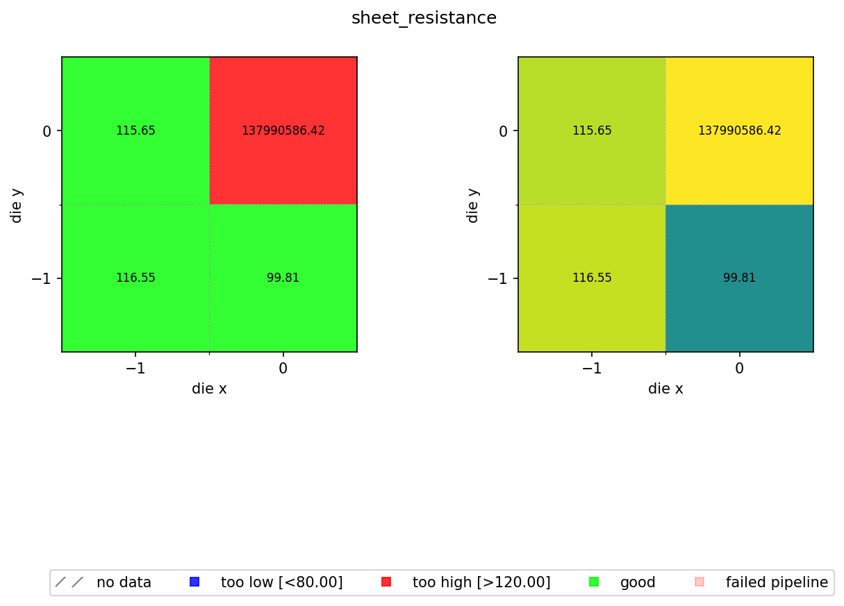
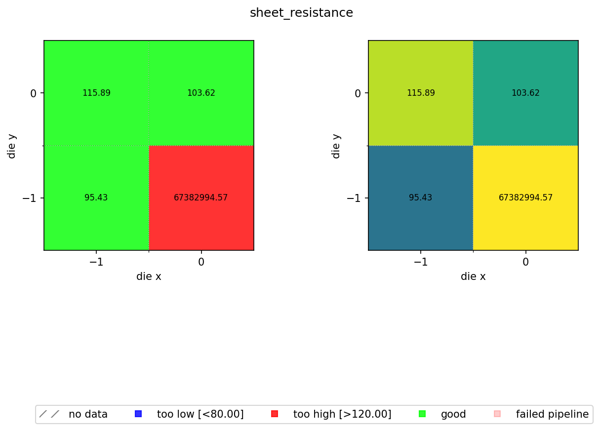
In the previous notebook we computed a sheet resistance estimate for every die on every wafer and stored the results as JSON files in DataLab. Now we aggregate those per-die results into a spatial wafer map so you can visualise process uniformity across the wafer.

The map colour-codes each die by pass/fail status against a spec range of 80 to 120 Ω/sq. A nominal sheet resistance of 100 Ω/sq with ±20% wafer variation and ±5% device variation means most dies should fall within this window. Dies outside the range are flagged blue (too low) or red (too high).

We reuse aggregate_die_analyses.py from the cutback series. That function reads JSON files containing die_x, die_y, and any scalar metric, and builds the two-panel pass/fail and continuous-colour wafer map.

Setup¶

import getpass
from pathlib import Path

import gfhub
from gfhub import nodes
from PIL import Image
from tqdm.notebook import tqdm

client = gfhub.Client()
user = getpass.getuser()
print(f"Running as user: {user}")

Running as user: runner

Upload the aggregation function¶

The aggregate_die_analyses.py script is shared across all tutorial series (cutback, resistance, rings, spirals). It reads the die_x, die_y, and the output_key field from each JSON file, places the values on a spatial grid, and renders the wafer map.

script = Path("../cutback/aggregate_die_analyses.py").read_text()
client.add_function(name="aggregate_die_analyses", function=script)
print("aggregate_die_analyses uploaded.")

aggregate_die_analyses uploaded.

Creating the pipeline¶

The spec limits for sheet resistance are 80 to 120 Ω/sq. The output_key must match the key written by die_sheet_resistance in notebook 4 ("sheet_resistance"). find_common_tags was uploaded in notebook 4. Because the pipeline reads all its inputs from DataLab and writes results back with provenance tags, the wafer map for any past run is always one query away.

p = gfhub.Pipeline()

p.trigger = nodes.on_manual_trigger()
p.load_file = nodes.load()
p.load_tags = nodes.load_tags()
p += p.trigger >> p.load_file
p += p.trigger >> p.load_tags

p.find_common_tags = nodes.function(function="find_common_tags")
p += p.load_tags >> p.find_common_tags

p.aggregate = nodes.function(
    function="aggregate_die_analyses",
    kwargs={
        "output_key": "sheet_resistance",
        "min_output": 80.0,
        "max_output": 120.0,
        "output_name": "wafer_sheet_resistance",
    },
)
p += p.load_file >> p.aggregate

p.save = nodes.save()
p += p.aggregate >> p.save[0]
p += p.find_common_tags >> p.save[1]

confirmation = client.add_pipeline(name="aggregate_die_analyses", schema=p)
print(f"Pipeline ready: {client.pipeline_url(confirmation['id'])}")

Pipeline ready: https://api.dev.gdsfactory.com/pipelines/019df3c3-407d-7530-b7a6-336d0e6f074a

Trigger per wafer¶

We query all die-level JSON files and group them by the wafer tag. The groupby works because wafer was set as a structured tag when each measurement was uploaded, so the list of wafers is discovered from the data itself rather than maintained in a separate config file.

entries = client.query_files(
    name="die_sheet_resistance.json",
    tags=[user, "project:tutorial_resistance", "wafer"],
).groupby("wafer")

job_ids = []
for wafer_tag, group in tqdm(entries.items()):
    print(f"Processing {wafer_tag}: {len(group)} dies")
    input_ids = [f["id"] for f in group]
    triggered = client.trigger_pipeline("aggregate_die_analyses", input_ids)
    job_ids.extend(triggered["job_ids"])

print(f"Triggered {len(job_ids)} wafer analysis jobs")

  0%|          | 0/2 [00:00<?, ?it/s]


Processing wafer:wafer1: 4 dies
Processing wafer:wafer2: 4 dies
Triggered 2 wafer analysis jobs

jobs = client.wait_for_jobs(job_ids)
print(f"All jobs complete. Statuses: {set(j['status'] for j in jobs)}")

  0%|          | 0/2 [00:00<?, ?it/s]


All jobs complete. Statuses: {'success'}

View the wafer maps¶

wafer_maps = client.query_files(
    name="wafer_sheet_resistance.png",
    tags=["project:tutorial_resistance", user],
)
print(f"Found {len(wafer_maps)} wafer maps")

for wm in wafer_maps:
    img = Image.open(client.download_file(wm["id"]))
    display(img)

Found 2 wafer maps