In the previous notebook we ran a per-die cutback fit and stored the extracted per-component loss in a JSON file for each die. Each JSON contains the die coordinates (die_x, die_y) and the fit results (component_loss, insertion_loss).
This notebook aggregates those die-level results into a spatial wafer map. That lets you see at a glance whether the MMI insertion loss is uniform across the wafer or whether there are systematic trends (radial gradients, edge effects, row-to-row variation) that point to process issues. Without the wafer tag shared across all die files, you would need to maintain a separate index or spreadsheet mapping each die result back to its wafer run. Here that mapping is implicit in the tags themselves, so the aggregation is a single groupby("wafer") call.
The map is produced by aggregate_die_analyses, a reusable function stored in this repository. It reads all the die JSON files for a wafer, plots the values on a grid, and colour-codes each die by pass/fail status against configurable spec limits.
Setup
import getpass
from pathlib import Path

import gfhub
from gfhub import nodes
from PIL import Image
from tqdm.notebook import tqdm

client = gfhub.Client()
user = getpass.getuser()
print(f"Running as user: {user}")
Running as user: runner
Uploading the aggregation function
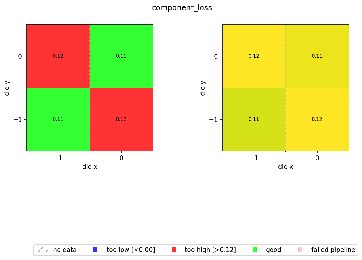
aggregate_die_analyses.py is a uv-script: a self-contained Python file with its own dependency block that DataLab can run directly without needing a separate gfhub.Function wrapper. It reads the JSON files produced by the die analysis pipeline, extracts die_x, die_y, and a configurable metric key, then builds a two-panel figure:
- Left panel: pass/fail map coloured by whether each die's value is within the spec limits (green = good, blue = too low, red = too high).
- Right panel: continuous colour scale showing the actual values, so you can see spatial trends within the passing population.
The function returns a single PNG path, which the pipeline saves to DataLab.
# Read the wafer analysis function from this directory and upload it
script = Path("aggregate_die_analyses.py").read_text()
client.add_function(name="aggregate_die_analyses", function=script)
print("aggregate_die_analyses uploaded.")
aggregate_die_analyses uploaded.
Creating the pipeline
The pipeline receives a group of die-analysis JSON files (one per die) and produces a single wafer map PNG. The find_common_tags function, uploaded in notebook 3, extracts the tags shared by all input files so the output is tagged with the wafer ID, project, and username without any die-specific tags leaking through. This means the wafer map is as queryable as any other file in DataLab: query_files(name="wafer_map.png", tags=["wafer:wafer_tutorial"]) will find it reliably, with no knowledge of where it was saved or who ran the analysis.
The min_output and max_output kwargs define the acceptable range for component_loss. Anything outside this range is flagged on the pass/fail map. Adjust these to match your process spec.
p = gfhub.Pipeline()

# Manual trigger only: we pass all dies from one wafer as a group
p.trigger = nodes.on_manual_trigger()

# Load all JSON files and their tags
p.load_file = nodes.load()
p.load_tags = nodes.load_tags()
p += p.trigger >> p.load_file
p += p.trigger >> p.load_tags

# Find the tags shared by all input die files (wafer, project, username)
p.find_common_tags = nodes.function(function="find_common_tags")
p += p.load_tags >> p.find_common_tags

# Aggregate all die JSONs into a wafer map PNG
p.aggregate = nodes.function(
    function="aggregate_die_analyses",
    kwargs={
        "output_key": "component_loss",
        "min_output": 0.0,
        "max_output": 0.115,
        "output_name": "wafer_map",
    },
)
p += p.load_file >> p.aggregate

# Save the wafer map with the common tags
p.save = nodes.save()
p += p.aggregate >> p.save[0]
p += p.find_common_tags >> p.save[1]

confirmation = client.add_pipeline(name="aggregate_die_analyses", schema=p)
print(f"Pipeline ready: {client.pipeline_url(confirmation['id'])}")
Pipeline ready: https://api.dev.gdsfactory.com/pipelines/019df3b7-b8ce-70d0-b501-88765c9c7ede
Triggering the wafer map per wafer
We query all die analysis JSON files, group them by wafer, and trigger the pipeline once per wafer. Each trigger call passes the full set of die JSON files for that wafer as a group, so the aggregation function sees all dies at once and can build the complete spatial map.
groupby("wafer") works here for the same reason groupby("die") worked in notebook 3: the wafer ID was set as a tag when each measurement file was uploaded, and every derived file (including the die JSON outputs) inherited it through the pipeline's shared-tag logic. There is no external lookup table needed to know which die belongs to which wafer run.
entries = client.query_files(
    name="cutback_die_analysis.json",
    tags=[user, "project:tutorial_cutback", "wafer"],
).groupby("wafer")

job_ids = []
for wafer_tag, group in tqdm(entries.items()):
    print(f"Processing {wafer_tag}: {len(group)} die analyses")
    input_ids = [f["id"] for f in group]
    triggered = client.trigger_pipeline("aggregate_die_analyses", input_ids)
    job_ids.extend(triggered["job_ids"])

print(f"Triggered {len(job_ids)} wafer analysis jobs")
  0%|          | 0/1 [00:00<?, ?it/s]


Processing wafer:wafer_tutorial: 4 die analyses
Triggered 1 wafer analysis jobs
jobs = client.wait_for_jobs(job_ids)
print(f"All jobs complete. Statuses: {[j['status'] for j in jobs]}")
  0%|          | 0/1 [00:00<?, ?it/s]


All jobs complete. Statuses: ['success']
Viewing the wafer map
wafer_maps = client.query_files(
    name="wafer_map.png",
    tags=["project:tutorial_cutback", user],
)

print(f"Found {len(wafer_maps)} wafer maps")

if wafer_maps:
    img = Image.open(client.download_file(wafer_maps[0]["id"]))
    display(img)
Found 1 wafer maps
What's next?
You have completed the cutback analysis series. The workflow you built here generalises to any metric that can be extracted from a group of per-device measurements and reduced to a single number per die. The aggregate_die_analyses.py function is shared with the resistance, rings, and spirals tutorial series, so you will see the same wafer map pattern reused there.