In the previous notebook we extracted a propagation loss value for each (die, waveguide type, width) combination. Now we aggregate the rib waveguide results into spatial wafer maps. Pulling together the right die JSONs for a given width would normally mean maintaining a folder structure or a spreadsheet that stays in sync with the files. Querying by tags and grouping server-side makes that step routine.
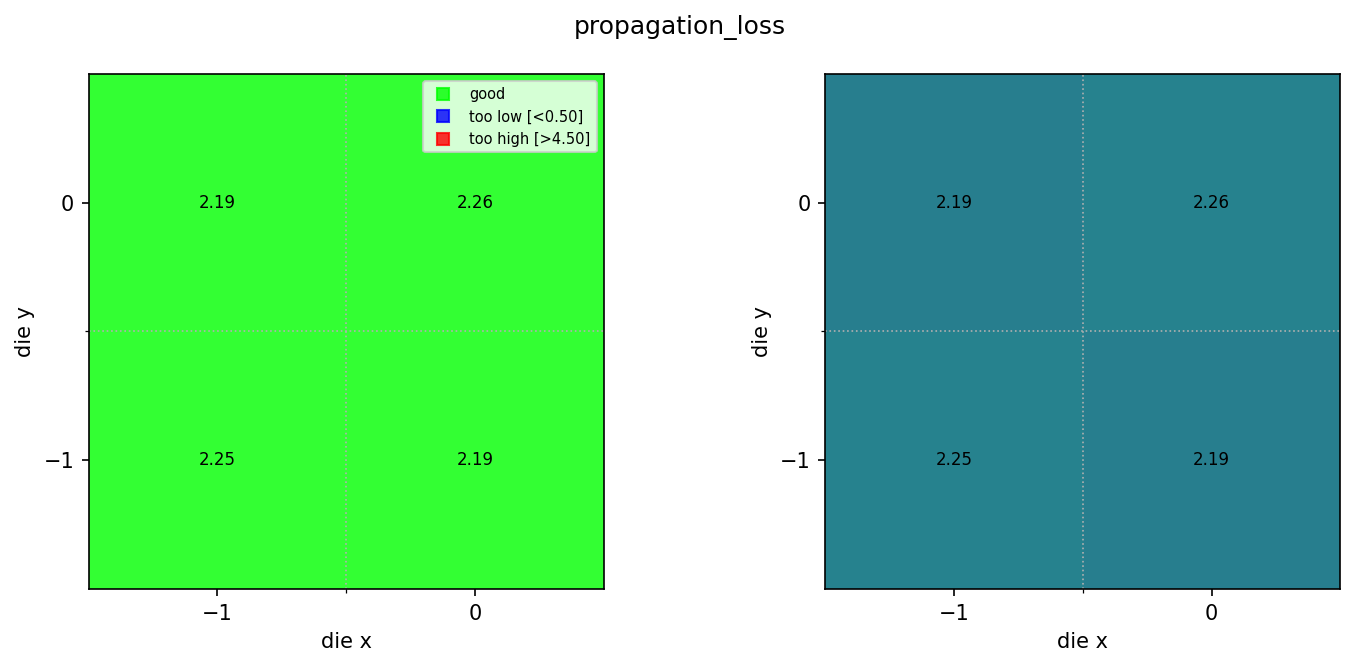
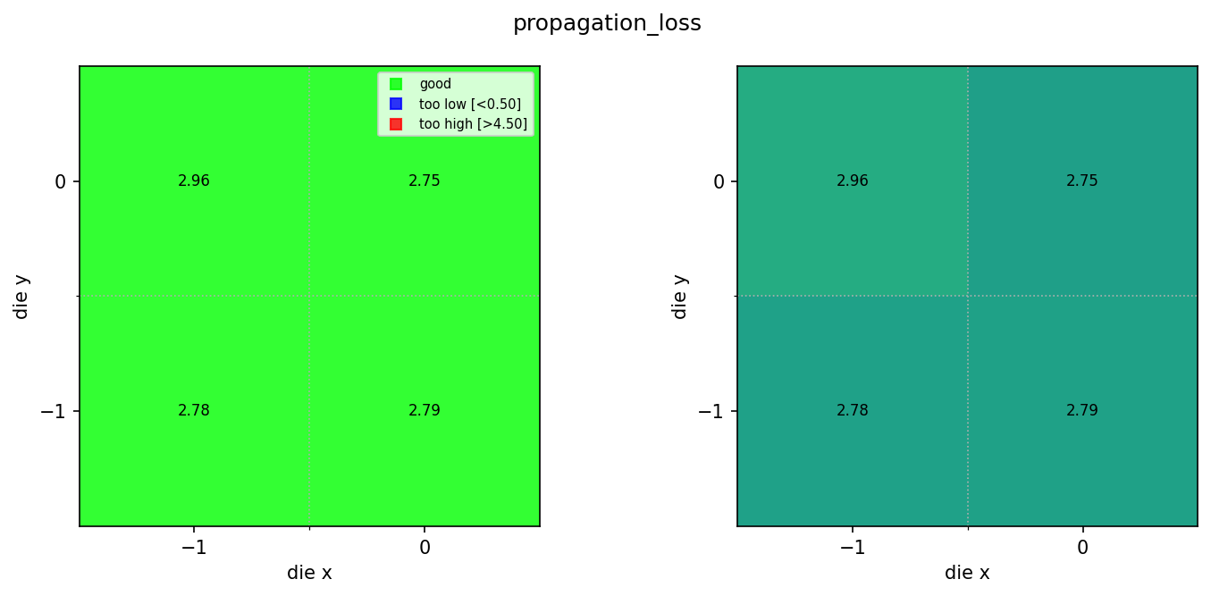
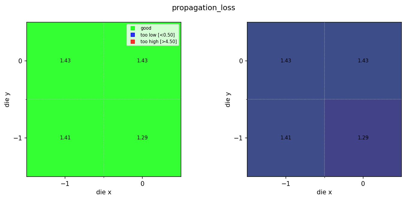
Because each waveguide width has its own characteristic propagation loss, we trigger one wafer map pipeline per (wafer, width) combination. The resulting maps let you see: - Whether propagation loss is uniform across the wafer. - Whether any dies fall outside the acceptable range (shown in red or blue on the pass-fail map). - Spatial gradients, such as edge vs. centre differences, that can indicate etch uniformity issues.
The spec limits here (0.5 to 4.5 dB/cm) are set to cover all three rib widths. For a production process you would define width-specific limits.
Setup
import getpass
from pathlib import Path

import gfhub
from gfhub import nodes
from PIL import Image
from tqdm.auto import tqdm

client = gfhub.Client()
user = getpass.getuser()
print(f"Running as user: {user}")
Running as user: runner
The wafer map function
spirals_wafer_map.py contains a function that reads per-die JSON files, extracts die coordinates and a configurable metric, and renders a two-panel figure:
- Left panel: pass/fail map — green for dies within spec, blue for too low, red for too high, hatched for missing.
- Right panel: continuous colour scale showing the actual values, so you can spot spatial gradients.
We import it, wrap it in gfhub.Function with its dependencies, and test it locally before uploading. The same function is reused in notebook 6 for ridge waveguides with different spec limits.
from spirals_wafer_map import main as spirals_wafer_map

func_def = gfhub.Function(
    spirals_wafer_map,
    dependencies={
        "json": "import json",
        "numpy": "import numpy as np",
        "matplotlib": [
            "import matplotlib.pyplot as plt",
            "import matplotlib.colors as mcolors",
        ],
    },
)
Testing locally
We download a sample group of die JSONs for one (wafer, width) combination and run .eval() to verify the function produces a correct wafer map before uploading.
import shutil

sample_entries = client.query_files(
    name="propagation_loss_rib_*.json",
    tags=["project:tutorial_spirals", user, "width_nm:500"],
)

sample_dir = Path("sample_wafer_map")
shutil.rmtree(sample_dir, ignore_errors=True)
sample_dir.mkdir()

sample_paths = [
    client.download_file(e["id"], sample_dir / f"{e['id']}.json")
    for e in sample_entries
]
print(f"Downloaded {len(sample_paths)} die JSONs")

result = func_def.eval(sample_paths, output_key="propagation_loss", min_output=0.5, max_output=4.5)
print(result)
Image.open(result["output"])
Downloaded 4 die JSONs


{'success': True, 'output': PosixPath('/home/runner/work/DataLab/DataLab/crates/sdk/examples/spirals/sample_wafer_map/wafer_map.png')}
spirals_wafer_map uploaded.
Creating the pipeline
The output_key is "propagation_loss" to match the field written by propagation_loss_from_cutback_spirals. The spec limits (0.5 to 4.5 dB/cm) are appropriate for rib waveguides across all three widths. The pipeline runs server-side, so any team member can trigger a fresh wafer map for a new lot without installing the analysis environment locally. find_common_tags was uploaded in notebook 4.
p = gfhub.Pipeline()

p.trigger = nodes.on_manual_trigger()
p.load_file = nodes.load()
p.load_tags = nodes.load_tags()
p += p.trigger >> p.load_file
p += p.trigger >> p.load_tags

p.find_common_tags = nodes.function(function="find_common_tags")
p += p.load_tags >> p.find_common_tags

p.aggregate = nodes.function(
    function="spirals_wafer_map",
    kwargs={
        "output_key": "propagation_loss",
        "min_output": 0.5,
        "max_output": 4.5,
    },
)
p += p.load_file >> p.aggregate

p.save = nodes.save()
p += p.aggregate >> p.save[0]
p += p.find_common_tags >> p.save[1]

confirmation = client.add_pipeline(name="rib_wafer_analysis", schema=p)
print(f"Pipeline ready: {client.pipeline_url(confirmation['id'])}")
Pipeline ready: https://api.dev.gdsfactory.com/pipelines/019df3c3-f798-7aa0-8c19-5f0f9d0e19df
Trigger per (wafer, width) group
We query the rib propagation loss JSONs and group by wafer and width. Grouping by (wafer, width_nm) works because both were set as tags when the die analysis results were saved. Without tags, collecting the right JSONs for each width across a full wafer would require parsing filenames or keeping a separate index. Each group triggers one wafer map job, so you get a separate map for each waveguide width.
entries = client.query_files(
    name="propagation_loss_rib_*.json",
    tags=["project:tutorial_spirals", user],
).groupby("wafer", "width_nm")

print(f"Found {len(entries)} (wafer, width) group(s)")

job_ids = []
for group_key, group in tqdm(entries.items()):
    print(f"  {group_key}: {len(group)} dies")
    input_ids = [f["id"] for f in group]
    triggered = client.trigger_pipeline("rib_wafer_analysis", input_ids)
    job_ids.extend(triggered["job_ids"])

print(f"Triggered {len(job_ids)} wafer analysis job(s)")
Found 3 (wafer, width) group(s)


  0%|          | 0/3 [00:00<?, ?it/s]


  ('wafer:wafer_tutorial', 'width_nm:500'): 4 dies
  ('wafer:wafer_tutorial', 'width_nm:800'): 4 dies
  ('wafer:wafer_tutorial', 'width_nm:300'): 4 dies
Triggered 3 wafer analysis job(s)
jobs = client.wait_for_jobs(job_ids)
print(f"All jobs complete. Statuses: {set(j['status'] for j in jobs)}")
  0%|          | 0/3 [00:00<?, ?it/s]


All jobs complete. Statuses: {'success'}
View the wafer maps
wafer_maps = client.query_files(
    name="wafer_map.png",
    tags=["project:tutorial_spirals", user, "waveguide_type:rib"],
)
print(f"Found {len(wafer_maps)} rib wafer maps")

for wm in wafer_maps:
    img = Image.open(client.download_file(wm["id"]))
    display(img)
Found 3 rib wafer maps

What's next?
The rib propagation loss wafer maps are ready. The next notebook creates the same maps for ridge waveguides. Ridge waveguides are expected to have higher propagation loss due to the full etch depth exposing more of the optical mode to sidewall roughness, so the spec limits are adjusted accordingly.