In the previous notebook we uploaded a sweep of simulated measurement spectra to DataLab, one file per die and device. Each file records the optical power versus wavelength for a specific cutback structure, tagged with the die coordinates, wafer ID, and component count.
Now we extract the actual per-component loss. The idea is straightforward: if you plot the peak transmitted power against the number of MMI repetitions for all structures on a single die, the result should be a straight line. The slope of that line is the loss per MMI in dB, and the intercept captures the fixed overhead from grating couplers and waveguide connections that is independent of device count.
In this notebook we:
- Load and explore the measurements for a single die to understand the data structure
- Define a
cutback_die_analysisfunction that runs the fit and saves a plot and a JSON summary - Define a
find_common_tagshelper that extracts shared provenance tags across a group of files - Wire both functions into a pipeline and trigger it independently for every die on the wafer
Setup
import getpass
import json
from pathlib import Path

import gfhub
import matplotlib.pyplot as plt
import numpy as np
import pandas as pd
from gfhub import nodes
from PIL import Image
from tqdm.notebook import tqdm

client = gfhub.Client()
user = getpass.getuser()
print(f"Running as user: {user}")
Running as user: runner
Exploring measurements for one die
Before building a function, it is worth loading the data interactively to see exactly what you are working with. We query all Parquet files tagged for die (-1,-1), download them, and reconstruct the tag strings from the entry metadata.
Tags on each file are stored as a dictionary mapping tag keys to objects that contain a parameter_value field when the tag carries a value. We flatten these back to strings of the form key:value or just key. The component count, die coordinates, and other metadata are all stored as tags, not inside the files themselves, so this reconstruction step is important for the analysis.
entries = client.query_files(
    tags=[
        user,
        "die:-1,-1",       # target a specific die
        "device",
        "project:tutorial_cutback",
        "cell",
        "wafer",
        ".parquet",
    ]
)
print(f"Found {len(entries)} files for die (-1,-1)")

# Download all files for this die
paths = [
    client.download_file(entry["id"], f"file_{i}.parquet")
    for i, entry in enumerate(entries)
]

# Reconstruct tag strings from the entry dict.
# Tags with a parameter_value become "key:value"; simple presence tags become just "key".
tags = [
    [
        (k if not (p := v.get("parameter_value")) else f"{k}:{p}")
        for k, v in entry["tags"].items()
    ]
    for entry in entries
]

print(f"Tags on first file: {tags[0]}")
Found 3 files for die (-1,-1)


Tags on first file: ['.parquet', 'project:tutorial_cutback', 'wafer:wafer_tutorial', 'die:-1,-1', 'cell:loss_0db', 'device:516.91,714.861', 'T:25.0', 'components:16', 'runner']
The cutback fit
For each file we take the peak measured power across the wavelength sweep. This acts as a proxy for the total transmitted power through that cutback structure, letting us compare the three different device lengths on a single number.
We then fit a straight line through the (component count, peak power) pairs using np.polyfit. The slope is the per-MMI insertion loss in dB, and the intercept captures the fixed losses from grating couplers, routing waveguides, and anything else that does not scale with the number of repetitions. Because more components means more loss (lower power), the slope comes out negative from polyfit and we flip its sign to report a positive loss value.
# Extract component count from tags (stored as "components:816", etc.)
num_comps = [
    int(next(t.replace("components:", "") for t in ts if t.startswith("components:")))
    for ts in tags
]

# Take the peak power across the wavelength axis for each file
powers = [pd.read_parquet(p)["power [dB]"].max() for p in paths]

# Linear fit. polyfit returns [slope, intercept]; both negated because loss reduces power.
component_loss, insertion_loss = [-float(x) for x in np.polyfit(num_comps, powers, deg=1)]

x = np.arange(0, max(num_comps) + 99, 100)
plt.scatter(num_comps, powers, color="C1", label="measured")
plt.plot(x, -component_loss * x - insertion_loss, color="C0", label="fit")
plt.grid(visible=True)
plt.xlim(x.min() - 30, x.max() + 30)
plt.title(f"Die (-1,-1): loss = {component_loss:.4f} dB/component")
plt.xlabel("# components")
plt.ylabel("Power [dB]")
plt.legend()
plt.show()

print(f"Loss per MMI:  {component_loss:.4f} dB")
print(f"Insertion loss at zero components: {insertion_loss:.4f} dB")
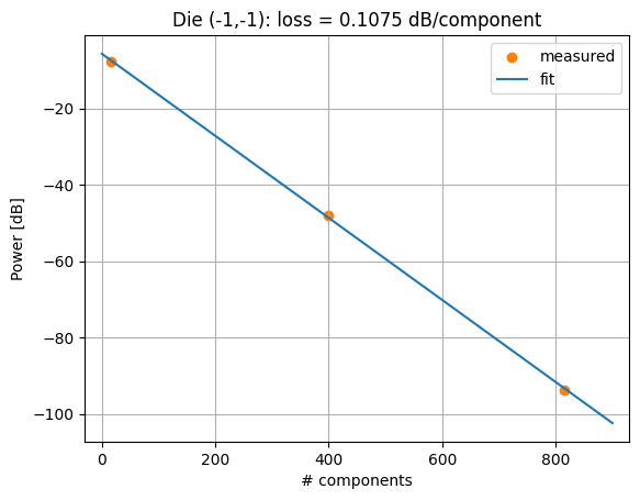
Loss per MMI:  0.1075 dB
Insertion loss at zero components: 5.6616 dB
Defining the analysis function
We now wrap the same logic into a DataLab function so it can run server-side for any die. The signature looks a bit different from the single-file functions in tutorial 3:
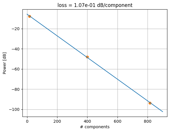
files: list[Path]andtags: list[list[str]]are the positional-only inputs. When the pipeline triggers this function with a group of file IDs, DataLab downloads all of them and passes the local paths as a list, along with the reconstructed tag strings in the same order.- The return type
tuple[Path, Path]means the function produces two output files: a PNG plot of the cutback fit, and a JSON file with the extracted loss values and die coordinates.
In the pipeline we will wire each output to its own save node using index notation (p.cutback_die_analysis[0] for the plot, [1] for the JSON).
def cutback_die_analysis(
    files: list[Path],
    tags: list[list[str]],
    /,
    *,
    output_name: str = "cutback_die_analysis",
) -> tuple[Path, Path]:
    """Run a cutback fit on a group of measurement files from a single die.

    Reads all Parquet files, extracts component counts from tags, fits a line
    through (components, peak power), and saves a plot and a JSON summary.
    """
    dfs = [pd.read_parquet(f) for f in files]

    # Component counts are stored as tags, not inside the files
    num_comps = [
        int(next(t.replace("components:", "") for t in ts if t.startswith("components:")))
        for ts in tags
    ]
    powers = [df["power [dB]"].max() for df in dfs]

    component_loss, insertion_loss = [
        -float(x) for x in np.polyfit(num_comps, powers, deg=1)
    ]

    x = np.arange(0, max(num_comps) + 99, 100)
    plt.scatter(num_comps, powers, color="C1")
    plt.plot(x, -component_loss * x - insertion_loss, color="C0")
    plt.grid(visible=True)
    plt.xlim(x.min() - 30, x.max() + 30)
    plt.title(f"loss = {component_loss:.2e} dB/component")
    plt.xlabel("# components")
    plt.ylabel("Power [dB]")

    path_plot = files[0].parent / f"{output_name}.png"
    plt.savefig(path_plot, bbox_inches="tight")
    plt.close()

    # Parse die coordinates from the first file's tags
    tag_dict = {k.split(":")[0]: k.split(":")[1] for k in tags[0] if ":" in k}
    die_x, die_y = [int(xy) for xy in tag_dict["die"].split(",")]

    output = {
        "die_x": die_x,
        "die_y": die_y,
        "component_loss": None if not np.isfinite(component_loss) else component_loss,
        "insertion_loss": None if not np.isfinite(insertion_loss) else insertion_loss,
    }
    path_json = files[0].parent / f"{output_name}.json"
    path_json.write_text(json.dumps(output))

    return path_plot, path_json
func_def = gfhub.Function(
    cutback_die_analysis,
    dependencies={
        "json": "import json",
        "numpy": "import numpy as np",
        "pandas[pyarrow]": "import pandas as pd",
        "matplotlib": "import matplotlib.pyplot as plt",
    },
)
Testing locally
We test the function using the files and tags we already downloaded in the exploration step. When the return type is a tuple, result["output"] is a list of file paths in the same order as the tuple elements.
result = func_def.eval(paths, tags)
print(result)  # {"success": True, "output": ["/path/to/plot.png", "/path/to/analysis.json"]}

Image.open(result["output"][0])
{'success': True, 'output': (PosixPath('/home/runner/work/DataLab/DataLab/crates/sdk/examples/cutback/cutback_die_analysis.png'), PosixPath('/home/runner/work/DataLab/DataLab/crates/sdk/examples/cutback/cutback_die_analysis.json'))}
cutback_die_analysis uploaded.
Tagging the outputs: find_common_tags
When we save the plot and JSON back to DataLab, we want them tagged with the provenance that was shared by all input files for this die: the wafer ID, die coordinates, project tag, and username. Tags that differ between files (such as cell name, component count, or device position) should not appear on the aggregate output, since the output represents the whole group, not any individual measurement.
find_common_tags solves this by collecting all tag values grouped by key, then keeping only keys where every file in the group agreed on the same value. File extension tags (keys starting with ., like .parquet) are excluded because the output files are a PNG and a JSON, not Parquet.
def find_common_tags(tags: list[list[str]], /) -> list[str]:
    """Return only the tags that are identical across all input files.

    Tags that vary between files are dropped. Extension tags (keys starting
    with '.') are always excluded regardless of whether they match.
    """
    # Build a dict mapping each tag key to the set of values seen across all files
    common: dict[str, set] = {}
    for _tags in tags:
        for t in _tags:
            if ":" in t:
                key, value = t.split(":", 1)
            else:
                key, value = t, ""
            common.setdefault(key, set()).add(value)

    # Keep only keys where all files agreed on the same value
    agreed = {k: next(iter(v)) for k, v in common.items() if len(v) == 1}

    # Reconstruct as tag strings, skipping extension keys
    return [
        k if not v else f"{k}:{v}"
        for k, v in agreed.items()
        if not k.startswith(".")
    ]
# Verify: die, wafer, and project should be shared; components and cell should not appear
common = find_common_tags(tags)
print(common)
['project:tutorial_cutback', 'wafer:wafer_tutorial', 'die:-1,-1', 'T:25.0', 'runner']
find_common_tags uploaded.
Creating the pipeline
This pipeline differs from the plot_parquet pipeline in notebook 2 in one important way: it has no auto-trigger on file upload. The cutback_die_analysis function needs all measurements from a die to be available at the same time to produce a meaningful fit. A single file upload cannot provide that, so we use only a manual trigger and fire it once all uploads are complete.
The pipeline:
- Receives a group of file IDs as a single trigger call
- Downloads all files and their tags
- Runs
cutback_die_analysisand gets back a plot path and a JSON path - Finds the tags shared by all input files
- Saves both outputs tagged with the shared provenance
Running the analysis as a pipeline rather than a local script matters because the function executes server-side from the registered definition. Any engineer on the team can trigger the same run and get the same result, without needing the analysis environment set up locally or having to locate the script themselves.
p = gfhub.Pipeline()

# Manual trigger only: the fit requires a full group of files, not a single upload
p.trigger = nodes.on_manual_trigger()

# Download all files in the group and their tags
p.load_file = nodes.load()
p.load_tags = nodes.load_tags()
p += p.trigger >> p.load_file
p += p.trigger >> p.load_tags

# Run the cutback fit: files go to input 0, tags go to input 1
p.cutback_die_analysis = nodes.function(function="cutback_die_analysis")
p += p.load_file >> p.cutback_die_analysis[0]
p += p.load_tags >> p.cutback_die_analysis[1]

# Find the tags shared by all input files, to attach to both outputs
p.common_tags = nodes.function(function="find_common_tags")
p += p.load_tags >> p.common_tags

# Save the plot (output 0) and the JSON (output 1), both with the shared tags
p.save_plot = nodes.save()
p += p.cutback_die_analysis[0] >> p.save_plot[0]
p += p.common_tags >> p.save_plot[1]

p.save_json = nodes.save()
p += p.cutback_die_analysis[1] >> p.save_json[0]
p += p.common_tags >> p.save_json[1]

confirmation = client.add_pipeline(name="cutback_die_analysis", schema=p)
print(f"Pipeline ready: {client.pipeline_url(confirmation['id'])}")
Pipeline ready: https://api.dev.gdsfactory.com/pipelines/019df3b5-bb8b-7a92-b8a5-7c37b4a46048
Triggering the analysis per die
groupby("die") partitions the query results by the value of the die tag, returning a dictionary where each key is a die coordinate string and each value is the list of entries from that die. We trigger the pipeline once per die, passing all its file IDs together as a group. DataLab then processes the group as a single job, and the pipeline receives all the files as a list.
This works because the die tag was set at upload time in notebook 2. There is no filename parser here and no separate mapping spreadsheet: the grouping key is already a structured attribute on every file, so groupby can partition the full dataset without any additional bookkeeping.
entries = client.query_files(
    tags=[user, "die", "device", "project:tutorial_cutback", "cell", "wafer", ".parquet"]
).groupby("die")

job_ids = []
for die_tag, group in tqdm(entries.items()):
    input_ids = [f["id"] for f in group]
    triggered = client.trigger_pipeline("cutback_die_analysis", input_ids)
    job_ids.extend(triggered["job_ids"])

print(f"Triggered {len(job_ids)} jobs")
  0%|          | 0/4 [00:00<?, ?it/s]


Triggered 4 jobs
jobs = client.wait_for_jobs(job_ids)
print(f"All jobs complete. Statuses: {[j['status'] for j in jobs]}")
  0%|          | 0/4 [00:00<?, ?it/s]


All jobs complete. Statuses: ['success', 'success', 'success', 'success']
What's next?
Each die now has a per-component loss estimate stored in DataLab as a JSON file, alongside a plot of the cutback fit. In the next notebook we load those JSON results, aggregate them across all dies on the wafer, and produce a spatial loss map that shows how device performance varies across the chip.