After a photomask comes back and wafers are processed, a cutback run typically produces one spectrum per component count per die per wafer. Those files land wherever the measurement software saves them, named by whatever convention was agreed on that day, and as soon as two engineers run the same measurement on different instruments the naming drifts and any batch query that relied on it breaks. The device table we build in this notebook is what replaces that convention: component count, die coordinates, and wafer ID become structured fields attached to the files themselves.
When you want to measure the insertion loss of a photonic device, say, a 1x2 MMI splitter, a single measurement is rarely enough. Fabrication variations, fiber coupling uncertainties, and waveguide losses all contribute to the total measured signal, making it hard to isolate the loss introduced by the device itself.
The cutback method solves this by measuring the same device cascaded a varying number of times in series. If you measure structures with 16, 400, and 816 MMIs in a row, the total loss scales linearly with the number of components. A linear fit to those measurements gives you the loss per MMI, cleanly separated from everything else.
This notebook shows you how to:
- Generate a cutback layout automatically using GDSFactory
- Upload the GDS file to DataLab
- Build a device table that records the position and component count of each structure on the chip.
- Upload that device table so later analysis pipelines can use it
Before you start, make sure your credentials are configured in
~/.gdsfactory/gdsfactoryplus.toml:
Setup
We capture the current system username. Files in DataLab are tagged with both project:tutorial_cutback and your username, so multiple users can run through this tutorial without overwriting each other's files or interfering with the real files.
import getpass
from itertools import chain
from pathlib import Path

import gdsfactory as gf
import gfhub
import pandas as pd
from gdsfactory.gpdk import PDK

PDK.activate()
client = gfhub.Client()
user = getpass.getuser()
print(f"Running as user: {user}")
Running as user: runner
Creating the cutback layout
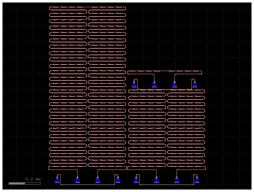
GDSFactory provides cutback_loss_mmi1x2, which automatically generates a sweep of cutback structures for a 1x2 MMI. We pass a list of loss values (one per cutback tier), where each value corresponds to a different number of MMI repetitions designed to span a target optical loss range.
Each structure then gets grating couplers added via add_fiber_array, which are the on-chip interfaces used to couple light in and out with a fiber probe during measurement.
gf.pack uses a 2D bin-packing algorithm to arrange the structures within the given reticle footprint (6050 x 4100 µm). It does not flatten or modify the cell hierarchy. It creates a new parent component that holds references to the originals, placed to minimize wasted space. If the structures do not all fit within a single reticle, gf.pack returns multiple bins, and gf.grid arranges those bins side by side into a regular grid. With this small sweep, everything fits in a single bin.
@gf.cell(check_ports=False)
def cutback() -> gf.Component:
    """Returns a component with a cutback sweep for loss measurement."""
    size = (6050, 4100)
    losses = (0, 1, 2)

    # Generate one cutback structure per loss value
    cutback_sweep = gf.components.cutback_loss_mmi1x2(
        component=gf.components.mmi1x2(), loss=losses
    )

    # Add fiber grating couplers for optical probing
    cutback_sweep_gratings = [gf.routing.add_fiber_array(c) for c in cutback_sweep]

    # Name each structure by its loss tier for easy identification
    for loss, c in zip(losses, cutback_sweep_gratings, strict=False):
        c.name = f"loss_{loss}db"

    # Pack all structures into the reticle footprint
    c = gf.pack(
        cutback_sweep_gratings, max_size=size, add_ports_prefix=False, spacing=2
    )
    c = gf.grid(c) if len(c) > 1 else c[0]
    return c


c = cutback()
c
Clean up existing files (optional)
If you have run this tutorial before, there may already be files in DataLab from a previous run. The cell below deletes any existing GDS and device table files that match your username and the project:tutorial_cutback tag, so you start fresh. Skip this cell if you want to keep previous uploads.
gds_files = client.query_files(name="cutback.gds", tags=["project:tutorial_cutback", user])
csv_files = client.query_files(
    name="cutback_device_table_example.csv", tags=["project:tutorial_cutback", user]
)
for file in chain(gds_files, csv_files):
    client.delete_file(file["id"])
    print(f"Deleted: {file['original_name']} ({file['id']})")
Deleted: cutback_device_table_example.csv (019df1ef-9042-73b0-8db2-3f966c1764e8)
Upload the GDS layout
We write the layout to a GDS file and upload it to DataLab. Tagging it with project:tutorial_cutback and your username means any later notebook in this series can find it with a simple query_files call, without needing to hardcode a file ID. The tags are what make this work: rather than encoding context into a directory path or a filename suffix, every attribute that matters for retrieval is a first-class queryable field that travels with the file regardless of where it is stored.
path = c.write_gds("cutback_example.gds")
uploaded = client.add_file(str(path), tags=["project:tutorial_cutback", user])
print(f"Uploaded GDS: {uploaded['original_name']} (id={uploaded['id']})")
Uploaded GDS: cutback_example.gds (id=019df3b5-5939-7992-a023-15a1f9ef96e1)
Building the device table
The layout contains multiple cutback structures placed at different positions on the chip. To analyse them later, we need to know where each structure sits and how many MMI components it contains. That is what the device table captures.
Each row corresponds to one cutback structure:
| Column | Description |
|---|---|
cell |
The cell name, e.g. loss_0db, loss_1db, loss_2db |
x, y |
Position of the structure on the reticle, in microns |
components |
Number of MMI repetitions in this structure |
cell_glob = "loss_*db"
info_keys = ("components",)

# GDSFactory cells expose a recursive instance iterator that walks the full
# cell hierarchy. Setting `targets` filters it to only visit cells whose
# name matches the given glob pattern, in this case our three cutback structures.
iterator = c.kdb_cell.begin_instances_rec()
iterator.targets = cell_glob

data = []
for _ in iterator:
    # Retrieve the child cell at this position in the hierarchy
    _c = c.kcl[iterator.inst_cell().cell_index()]

    # Compute the absolute position of this instance on the reticle.
    # Multiplying the two transformations gives the final placement relative
    # to the top-level cell. `.disp` is the translation vector; multiplying
    # by `dbu` converts from integer database units to microns.
    _disp = (iterator.trans() * iterator.inst_trans()).disp
    row = [_c.name, _disp.x * _c.kcl.dbu, _disp.y * _c.kcl.dbu]

    # GDSFactory stores metadata on each cell at creation time.
    # `components` holds the number of MMI repetitions in this structure.
    info = _c.info.model_dump()
    for key in info_keys:
        row.append(info.get(key))
    data.append(row)

df = pd.DataFrame(data=data, columns=["cell", "x", "y", *info_keys])
df
| cell | x | y | components | |
|---|---|---|---|---|
| 0 | loss_2db | 33.835 | 116.310 | 816 |
| 1 | loss_1db | 529.485 | 116.310 | 400 |
| 2 | loss_0db | 516.910 | 714.861 | 16 |
Upload the device table
We save the device table as a CSV and upload it to DataLab with the same tags as the GDS. Later notebooks in this series will query it by name and tags to load the structure positions and component counts for analysis. Because the tags travel with the file, those notebooks never need to know the file's path or ID in advance.
csv_path = Path("cutback_device_table_example.csv")
df.to_csv(csv_path, index=False)
uploaded_csv = client.add_file(csv_path, tags=["project:tutorial_cutback", user])
print(f"Uploaded device table: {uploaded_csv['original_name']} (id={uploaded_csv['id']})")
csv_path.unlink(missing_ok=True)
Uploaded device table: cutback_device_table_example.csv (id=019df3b5-5e3c-7da3-8aa0-876a27852b4e)
What's next?
You now have two files in DataLab: the GDS layout and the device table. The next notebook in this series shows how to upload your measurement data and associate it with the structures defined in this device table.