In the previous notebook each spiral device got a single number: the transmitted power at 1550 nm. Now we aggregate those per-device measurements to the die level and extract the propagation loss. Assembling the right files for each fit group is the step that normally requires either careful filename parsing or a separate lookup table. Here we query by tags and let the grouping happen on the server.
The physical model is straightforward. For a waveguide of length L:
P(L) [dBm] = P0 [dBm] - alpha [dB/cm] * L [cm]
where P0 is the power at zero length (set entirely by the grating coupler insertion loss) and alpha is the propagation loss we want to measure. A linear fit of P_dBm vs. L gives alpha as the magnitude of the slope.
The grouping key is (die, waveguide type, width). We cannot mix widths, because each width has a different loss. We cannot mix waveguide types either (rib and ridge have different etch depths and different loss values). Each group provides six points (one per spiral length, from 0 to 25 mm), which is enough for a reliable linear fit.
The function also extracts the grating coupler insertion loss from the fit intercept at L = 0, which is useful for process monitoring independent of waveguide loss.
Setup
import getpass
import json
import shutil
from pathlib import Path

import gfhub
import matplotlib.pyplot as plt
import numpy as np
from gfhub import nodes
from PIL import Image
from tqdm.auto import tqdm

client = gfhub.Client()
user = getpass.getuser()
print(f"Running as user: {user}")
Running as user: runner
Load sample data
We download the device analysis JSONs for one (die, type, width) group to verify the data before defining the pipeline function.
entries = client.query_files(
    name="*_analysis.json",
    tags=["project:tutorial_spirals", user, "die:0,0", "waveguide_type:rib", "width_nm:500"],
)
tags = [
    [gfhub.tags.into_string(t) for t in entry["tags"].values()]
    for entry in entries
]

sample_dir = Path("sample_die")
shutil.rmtree(sample_dir, ignore_errors=True)
sample_dir.mkdir()

sample_paths = []
for entry in entries:
    dest = sample_dir / f"{entry['id']}.json"
    client.download_file(entry["id"], dest)
    sample_paths.append(dest)

print(f"Downloaded {len(sample_paths)} files for die (0,0), rib, 500 nm")
print("Sample tags:", tags[0])
Downloaded 12 files for die (0,0), rib, 500 nm
Sample tags: ['project:tutorial_spirals', 'wafer:wafer_tutorial', 'die:0,0', 'cell:cutback_rib_assembled_MFalse_W0p5_L0', '.json', 'runner', 'waveguide_type:rib', 'width_nm:500', 'length_um:0']
Defining the die-level propagation loss function
propagation_loss_from_cutback_spirals receives all the device analysis JSON files for one (die, waveguide type, width) group. It reads power_dBm from each JSON and reads length_um from the file's tags (not from inside the JSON), then performs a linear fit.
The slope of the fit is in dB/µm. We multiply by 1e4 to convert to dB/cm, then negate to get a positive loss value.
The waveguide type and width are also read from tags so the output filenames and plot titles are descriptive.
def propagation_loss_from_cutback_spirals(
    files: list[Path],
    tags: list[list[str]],
    /,
) -> tuple[Path, Path]:
    """Fit propagation loss from spiral measurements at different lengths.

    Reads power_dBm from each JSON file and length_um from the corresponding tags,
    then fits P_dBm = P0 - alpha * L to extract alpha in dB/cm.
    """
    # Collect (length_um, power_dBm) pairs from files and their tags
    lengths_um = []
    powers_dBm = []
    for file, file_tags in zip(files, tags):
        data = json.loads(file.read_text())
        power_dBm = data.get("power_dBm")
        if power_dBm is None:
            continue
        length_um = next(
            (float(t.split(":", 1)[1]) for t in file_tags if t.startswith("length_um:")),
            None,
        )
        if length_um is not None:
            lengths_um.append(length_um)
            powers_dBm.append(power_dBm)

    if len(lengths_um) < 2:
        msg = "Need at least 2 measurements for a propagation loss fit"
        raise ValueError(msg)

    lengths_um = np.array(lengths_um)
    powers_dBm = np.array(powers_dBm)

    # Sort by length so the plot looks clean
    order = np.argsort(lengths_um)
    lengths_um = lengths_um[order]
    powers_dBm = powers_dBm[order]

    # Linear fit: slope is in dB/µm, convert to dB/cm
    coeffs = np.polyfit(lengths_um, powers_dBm, deg=1)
    slope_dB_per_um = coeffs[0]  # negative value
    intercept_dBm = coeffs[1]    # grating coupler reference power at L=0
    alpha_dBcm = -slope_dB_per_um * 1e4  # propagation loss in dB/cm

    # R-squared of the fit
    fitted = np.polyval(coeffs, lengths_um)
    ss_res = float(np.sum((powers_dBm - fitted) ** 2))
    ss_tot = float(np.sum((powers_dBm - powers_dBm.mean()) ** 2))
    r_squared = 1.0 - ss_res / ss_tot if ss_tot > 0 else 0.0

    # Read die coordinates, width, and waveguide type from the first file's tags
    die_x, die_y = None, None
    width_nm = None
    waveguide_type = None
    for t in tags[0]:
        if t.startswith("die:"):
            die_x, die_y = [int(v) for v in t.split(":", 1)[1].split(",")]
        elif t.startswith("width_nm:"):
            width_nm = int(t.split(":", 1)[1])
        elif t.startswith("waveguide_type:"):
            waveguide_type = t.split(":", 1)[1]

    fig, ax = plt.subplots(figsize=(8, 5))
    ax.scatter(lengths_um * 1e-4, powers_dBm, s=60, zorder=5, label="measured")
    length_fit = np.linspace(0, lengths_um.max(), 100)
    ax.plot(
        length_fit * 1e-4,
        np.polyval(coeffs, length_fit),
        "r--",
        label=f"fit: {alpha_dBcm:.2f} dB/cm  (R²={r_squared:.3f})",
    )
    ax.set_xlabel("Length (cm)")
    ax.set_ylabel("Power (dBm)")
    ax.set_title(
        f"Die ({die_x}, {die_y}), {waveguide_type}, {width_nm} nm — propagation loss"
    )
    ax.legend()
    ax.grid(True, alpha=0.3)
    plt.tight_layout()

    stem = f"propagation_loss_{waveguide_type}_{width_nm}nm"
    plot_path = files[0].parent / f"{stem}.png"
    plt.savefig(plot_path, bbox_inches="tight", dpi=100)
    plt.close()

    results = {
        "die_x": die_x,
        "die_y": die_y,
        "propagation_loss": float(alpha_dBcm),
        "r_squared": float(r_squared),
        "grating_coupler_loss_dBm": float(intercept_dBm),
        "num_devices": len(lengths_um),
        "width_nm": width_nm,
        "waveguide_type": waveguide_type,
    }
    results_path = files[0].parent / f"{stem}.json"
    results_path.write_text(json.dumps(results, indent=2))

    return plot_path, results_path
func_def = gfhub.Function(
    propagation_loss_from_cutback_spirals,
    dependencies={
        "json": "import json",
        "numpy": "import numpy as np",
        "matplotlib": "import matplotlib.pyplot as plt",
    },
)
Testing locally
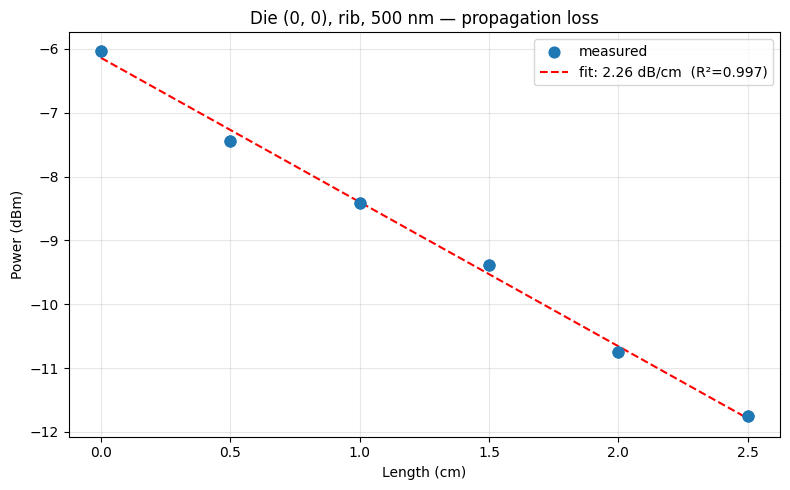
We test the function on the sample files downloaded above. This runs the function in a sandboxed uv environment with func_def.eval(), the same way it will run on the server. For a tuple-return function, result["output"] is a list with one element per return value. The plot should show a clear downward trend of power vs. length, with the fit line capturing the propagation loss slope.
result = func_def.eval(sample_paths, tags)
plot_path, json_path = result["output"]
print(json_path.read_text())
Image.open(plot_path)
{
  "die_x": 0,
  "die_y": 0,
  "propagation_loss": 2.2581782174984606,
  "r_squared": 0.996783162539795,
  "grating_coupler_loss_dBm": -6.140679357450991,
  "num_devices": 12,
  "width_nm": 500,
  "waveguide_type": "rib"
}
propagation_loss_from_cutback_spirals uploaded.
Common tags
The outputs for each (die, type, width) group should be tagged with the provenance shared by all devices in that group: die, waveguide_type, width_nm, wafer, and project. Tags that vary between devices — in particular length_um and cell — should not appear on the aggregated output. find_common_tags handles this by keeping only tags where every input file agrees on the same value. Extension tags (keys starting with .) are always excluded.
This is the same helper used in the cutback, resistance, and rings series. It is re-uploaded here so this tutorial can be followed independently.
def find_common_tags(tags: list[list[str]], /) -> list[str]:
    """Return only the tags that are identical across all input files."""
    common: dict[str, set] = {}
    for _tags in tags:
        for t in _tags:
            if ":" in t:
                key, value = t.split(":", 1)
            else:
                key, value = t, ""
            common.setdefault(key, set()).add(value)
    agreed = {k: next(iter(v)) for k, v in common.items() if len(v) == 1}
    return [k if not v else f"{k}:{v}" for k, v in agreed.items() if not k.startswith(".")]


client.add_function(find_common_tags)
print("find_common_tags uploaded.")
find_common_tags uploaded.
Creating the pipeline
This pipeline uses a manual trigger only. There is no meaningful auto-trigger here because the pipeline needs a group of files (all lengths for one die and width), not a single file. The function is registered server-side, so re-running the fit for a new wafer does not require anyone to re-upload or re-configure the analysis. Grouping happens in the trigger loop below, where we pass a list of file IDs per group.
p = gfhub.Pipeline()

p.trigger = nodes.on_manual_trigger()
p.load_file = nodes.load()
p.load_tags = nodes.load_tags()
p += p.trigger >> p.load_file
p += p.trigger >> p.load_tags

p.propagation_loss = nodes.function(function="propagation_loss_from_cutback_spirals")
p += p.load_file >> p.propagation_loss[0]
p += p.load_tags >> p.propagation_loss[1]

p.common_tags = nodes.function(function="find_common_tags")
p += p.load_tags >> p.common_tags

p.save_plot = nodes.save()
p.save_json = nodes.save()
p += p.propagation_loss[0] >> p.save_plot[0]
p += p.common_tags >> p.save_plot[1]
p += p.propagation_loss[1] >> p.save_json[0]
p += p.common_tags >> p.save_json[1]

confirmation = client.add_pipeline(name="spiral_propagation_loss", schema=p)
print(f"Pipeline ready: {client.pipeline_url(confirmation['id'])}")
Pipeline ready: https://api.dev.gdsfactory.com/pipelines/019df3c3-359a-7532-9703-0bc913a30bd1
Trigger per (die, waveguide type, width) group
We group the device analysis JSONs by all three dimensions at once. Grouping by (die, waveguide_type, width_nm) works because all three were set as tags at upload time. Without tags, assembling the right files for each fit group would require parsing filenames or querying a separate database. Each group has six files (one per spiral length), and each group gets its own pipeline job.
analysis_files = client.query_files(
    name="*_analysis.json",
    tags=["project:tutorial_spirals", user],
).groupby("die", "waveguide_type", "width_nm")

print(f"Found {len(analysis_files)} (die, type, width) groups")

job_ids = []
for group_key, files in tqdm(analysis_files.items()):
    input_ids = [f["id"] for f in files]
    triggered = client.trigger_pipeline("spiral_propagation_loss", input_ids)
    job_ids.extend(triggered["job_ids"])

print(f"Triggered {len(job_ids)} die analysis jobs")
Found 24 (die, type, width) groups


  0%|          | 0/24 [00:00<?, ?it/s]


Triggered 24 die analysis jobs
jobs = client.wait_for_jobs(job_ids)
print(f"All jobs complete. Statuses: {set(j['status'] for j in jobs)}")
  0%|          | 0/24 [00:00<?, ?it/s]


All jobs complete. Statuses: {'success'}
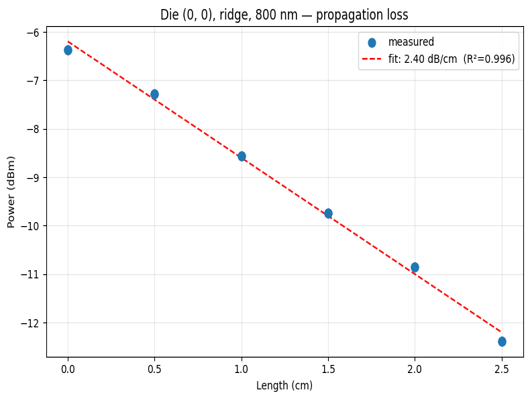
View a sample result
die_plots = client.query_files(name="propagation_loss_*.png", tags=["project:tutorial_spirals", user])
print(f"Found {len(die_plots)} propagation loss plots")

if die_plots:
    img = Image.open(client.download_file(die_plots[0]["id"]))
    display(img.resize((530, 400)))
Found 24 propagation loss plots
What's next?
Each (die, waveguide type, width) combination now has a JSON with the fitted propagation loss in dB/cm and the die coordinates. Notebooks 5 and 6 aggregate these into spatial wafer maps — notebook 5 for rib waveguides, notebook 6 for ridge waveguides — so you can see whether loss is uniform across the wafer or shows a systematic gradient.