CPW parametric amplifiers: layout and circuit models
Required extras
Needs
modelsand the external VACASK simulator:uv sync --extra models(orpip install "qpdk[models]"). Install VACASK, putvacaskonPATHor setVACASK; it compiles Verilog-A with the bundledopenvaf-r, and Linux also needsbinutils. See the extras reference.
A flux-pumped JPA uses a SQUID to modulate the resonance of a distributed resonator at twice its frequency Yamamoto et al. (2008). To simulate that in a circuit solver, represent the linear part as a subcircuit and solve the pumped nonlinear part with harmonic balance Kundert et al. (1986), Maas (2003).
This notebook checks the models with released VACASK. It compares two line models against SAX. It then uses them to measure resonance against flux, the single-mode threshold, gain against pump amplitude, and the higher-mode conversion that breaks the simple signal-idler balance. The TWPA notebook covers traveling-wave amplification. The lumped companion runs lumped Kerr and SQUID examples.
The analyses differ in what they assume. AC linearizes the circuit around its DC operating point. ACSP returns S-parameters with the pump off. HB finds the nonlinear periodic pump. HBAC finds infinitesimal signal and idler waves around that pump. The Choose a VACASK analysis in the lumped companion compares them in detail.
Show code
import os
import time
from pathlib import Path

import jax
import jax.numpy as jnp
from jax.typing import ArrayLike
from matplotlib import font_manager, pyplot as plt
from matplotlib.collections import PolyCollection
from sax.models import rf

import qpdk.colormaps  # ruff: ignore[unused-import] - registers the style colormap
from qpdk import PDK, logger
from qpdk.cells.resonator import resonator
from qpdk.config import PATH
from qpdk.models.constants import Φ_0
from qpdk.models.cpw import get_cpw_dimensions, get_cpw_substrate_params
from qpdk.models.junction import squid_junction
from qpdk.simulation.vacask import (
    Netlist,
    Vacask,
    VacaskError,
    cpw_tline_params,
    format_value,
    vector_fit,
    vector_fit_subckt,
)

# Agg suppresses notebook figure outputs in headless CI.
if "ipykernel" in sys.modules:
    from IPython import get_ipython
    from matplotlib_inline.backend_inline import set_matplotlib_formats

    if (ipython := get_ipython()) is not None:
        ipython.run_line_magic("matplotlib", "inline")
        set_matplotlib_formats("png", "svg")

jax.config.update("jax_enable_x64", True)
PDK.activate()

# The checkout stylesheet is absent from installed wheels.
for _style in (PATH.docs / "qpdk.mplstyle", "qpdk"):
    try:
        plt.style.use(_style)
    except OSError:
        continue
    break

# The stylesheet names fonts that only the docs build ships; register them so
# they resolve without docs/ipython_config.py.
_font_dir = os.environ.get("QPDK_DOCS_FONTS_DIR")
for _fonts in (Path(_font_dir) if _font_dir else None, PATH.repo / "build/docs-fonts"):
    if _fonts is not None and _fonts.is_dir():
        for _font in sorted(_fonts.iterdir()):
            if _font.suffix in {".otf", ".ttf"}:
                font_manager.fontManager.addfont(str(_font))
        break
Finding VACASK
Vacask.find() <qpdk.simulation.vacask.Vacask.find> checks the
VACASK/QPDK_VACASK environment variables and PATH. The notebook stops
if the binary is missing.
try:
    vacask = Vacask.find()
except VacaskError as error:
    print(error)
    raise SystemExit(
        "VACASK is not installed; skipping the rest of this notebook."
    ) from None
print(f"Using VACASK at {vacask.binary}")
Every netlist uses tolscale=1e-6 reltol=1e-6. The default tolerances shift
the gain by more than the differences resolved here. Port conventions:
- A port is a Norton source \(I_\text{s}\) in parallel with \(R=50\,\Omega\). So \(V_\text{inc}=I_\text{s}R/2\) and \(\Gamma=2V/(I_\text{s}R)-1\) Pozar (2012).
- VACASK reports a
sinesource of amplitude \(A\) as \(-\text{j}A\), so the incident HB phasor is \(-\text{j}I_\text{s}R/2\). hbacwrites the response at \(f_\text{s}+k f_\text{p}\) asnode;k.
R_PORT = 50.0
I_SIG = 1e-9
OPTIONS = "options tolscale=1e-6 reltol=1e-6"
SMALL_SIGNAL = f"mag=1e-9 spur={{[0]}} smag=[{I_SIG}]"


def db(x: ArrayLike) -> jax.Array:
    r"""Power gain in dB of a wave amplitude ratio, $20\log_{10}|A|$. See :cite:p:`m.pozarMicrowaveEngineering2012`."""
    return 20 * jnp.log10(jnp.abs(x))


def reflection(v: ArrayLike, source_current: float) -> jax.Array:
    r"""Reflection coefficient of a Norton port from its node voltage.

    Uses $\Gamma=2V/(I_\text{s}R)-1$
    :cite:p:`m.pozarMicrowaveEngineering2012`.

    Returns:
        Complex reflected wave amplitude divided by the incident amplitude.
    """
    return 2 * jnp.asarray(v) / (source_current * R_PORT) - 1


def conversion(v: ArrayLike, source_current: float) -> jax.Array:
    r"""Conversion gain into a sideband other than the one driven.

    The sideband amplitude is $2V/(I_\text{s}R)$, as in
    frequency-conversion analysis :cite:p:`maasNonlinearMicrowaveRF2003`.

    Returns:
        Complex sideband wave amplitude divided by the incident amplitude.
    """
    return 2 * jnp.asarray(v) / (source_current * R_PORT)


def show_plot() -> None:
    """Show the current figure with Outfit titles, as the docs config does."""
    fig = plt.gcf()
    for text in [ax.title for ax in fig.axes] + list(fig.texts):
        if text.get_text():
            text.set_fontfamily("Outfit")
            text.set_fontweight("bold")
    plt.show()
SQUID-terminated quarter-wave resonator
Following {cite:t}yamamotoFluxdrivenJosephsonParametric2008, a 4680 µm CPW
(\(\lambda/4\) at 6.5 GHz) is shorted through the SQUID. It is coupled to the
port by \(C_\text{c}=20\) fF, using the PDK cpw cross-section. The pump
modulates the SQUID flux at \(f_\text{p}\approx2f_0\). A signal at
\(f_\text{s}\) is amplified with an idler at \(f_\text{p}-f_\text{s}\). This is
three-wave mixing.
The symmetric SQUID is one junction with \(I_\text{c,tot}\cos(\pi\Phi/\Phi_0)\). This neglects loop inductance, valid for \(\beta_L=2L_\text{loop}I_\text{c}/\Phi_0\ll1\) Tesche et al. (1977). Its flux terminal is driven in units of \(\Phi_0\).
Use the same geometry for layout and models
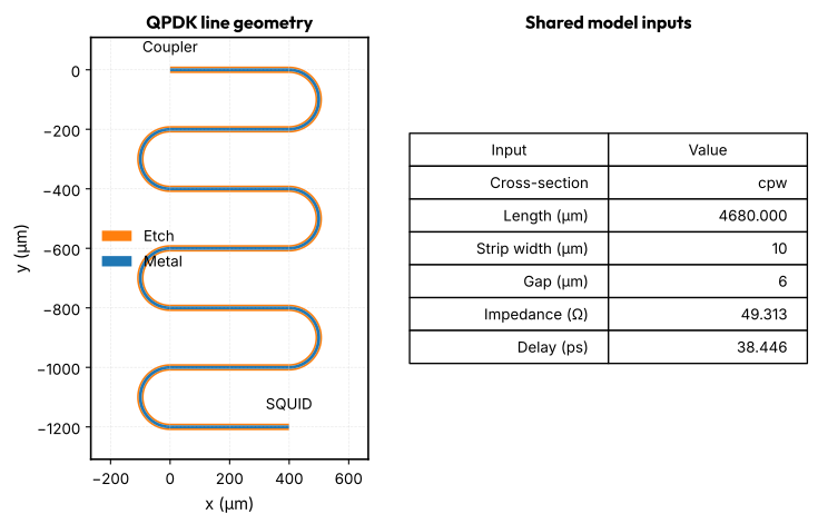
Make a QPDK meander with the cpw cross-section. Read its realized centreline length after grid snapping. Use that length and cross-section for both the SAX line model and VACASK's line impedance and delay. Here the realized length is 4680 µm, the strip width is 10 µm and the gap is 6 µm.
The two end ports connect to the ideal coupling capacitor and SQUID in the circuit. Those end devices are not drawn here. The line model uses a uniform cross-section approximation Simons (2001), Ghione et al. (1984). It does not include coupling between meanders, bend corrections or end-pad parasitics. For those effects, export this geometry to a field solver as in the CPW field simulation notebook.
The plot below comes from the layout polygons. Changing the cross-section or length changes both the geometry and the model inputs.
LINE_CROSS_SECTION = "cpw"
line_layout = resonator(
    length=4680.0,
    meanders=6,
    cross_section=LINE_CROSS_SECTION,
    open_start=False,
    open_end=False,
)
LENGTH = float(line_layout.info["length"])
C_COUPLING = 20e-15
width, gap = get_cpw_dimensions(LINE_CROSS_SECTION)
h_sub, t_metal, ep_r, _ = get_cpw_substrate_params()
z0_line, td_line = cpw_tline_params(LENGTH, cross_section=LINE_CROSS_SECTION)
logger.info(
    "Layout length {} µm, Z0 {:.4f} Ω, delay {:.4f} ps", LENGTH, z0_line, td_line * 1e12
)

fig, (ax_layout, ax_values) = plt.subplots(
    1, 2, figsize=(8, 5), gridspec_kw={"width_ratios": [1, 1.2]}
)
polygons = line_layout.get_polygons_points(by="name")
for layer_name, color, label in (
    ("M1_ETCH", "C1", "Etch"),
    ("M1_DRAW", "C0", "Metal"),
):
    ax_layout.add_collection(
        PolyCollection(
            polygons[layer_name], facecolor=color, edgecolor="none", label=label
        )
    )
for port_name, label in (("o1", "Coupler"), ("o2", "SQUID")):
    port = line_layout.ports[port_name]
    ax_layout.annotate(
        label, port.center, xytext=(0, 12), textcoords="offset points", ha="center"
    )
ax_layout.autoscale_view()
ax_layout.margins(0.25, 0.08)
ax_layout.set_aspect("equal")
ax_layout.set(xlabel="x (µm)", ylabel="y (µm)", title="QPDK line geometry")
ax_layout.legend(loc="center left", bbox_to_anchor=(0, 0.5))
ax_values.axis("off")
parameters = [
    ["Cross-section", LINE_CROSS_SECTION],
    ["Length (µm)", f"{LENGTH:.3f}"],
    ["Strip width (µm)", f"{width:g}"],
    ["Gap (µm)", f"{gap:g}"],
    ["Impedance (Ω)", f"{z0_line:.3f}"],
    ["Delay (ps)", f"{td_line * 1e12:.3f}"],
]
parameter_table = ax_values.table(
    cellText=parameters, colLabels=["Input", "Value"], loc="center"
)
parameter_table.auto_set_font_size(False)
parameter_table.set_fontsize(10)
parameter_table.scale(1, 1.8)
ax_values.set_title("Shared model inputs")
fig.tight_layout()
show_plot()
2026-10-21 10:06:40.902 | INFO     | __main__:<module>:14 - Layout length 4680.0 µm, Z0 49.3128 Ω, delay 38.4457 ps
findfont: Failed to find font weight bold, now using 400.
A distributed line and a rational fit
- Route A: an ideal
tline_idealwith \(Z_0\) and delay fromcpw_tline_params. This is exact for a lossless TEM line. - Route B: a rational fit of any linear SAX model by
vector_fit(vector fitting with passivity enforcement Gustavsen et al. (1999)), emitted byvector_fit_subckt.
Both are compared with SAX after renormalizing to 50 Ω through ABCD matrices Pozar (2012). The loss tangent is zero, so all three describe the same lossless line.
The line comparison and the fit check answer different questions. The CPW dispersion comes from the SAX coplanar-waveguide model Göppl et al. (2008). The rational fit tests only how well Route B reproduces that model.
def s_to_abcd(s: jax.Array, z0: float) -> jax.Array:
    """ABCD matrices of two-port S-matrices ``(..., 2, 2)`` referenced to ``z0``.

    Standard S-to-ABCD conversion :cite:p:`m.pozarMicrowaveEngineering2012`.

    Returns:
        ABCD matrices with the same leading axes as the input.
    """
    s11, s12, s21, s22 = s[..., 0, 0], s[..., 0, 1], s[..., 1, 0], s[..., 1, 1]
    a = ((1 + s11) * (1 - s22) + s12 * s21) / (2 * s21)
    b = z0 * ((1 + s11) * (1 + s22) - s12 * s21) / (2 * s21)
    c = ((1 - s11) * (1 - s22) - s12 * s21) / (2 * s21 * z0)
    d = ((1 - s11) * (1 + s22) + s12 * s21) / (2 * s21)
    return jnp.stack([jnp.stack([a, b], -1), jnp.stack([c, d], -1)], -2)


def abcd_to_s(abcd: jax.Array, z0: float) -> jax.Array:
    """Two-port S-matrices of ABCD matrices, referenced to ``z0``.

    Standard ABCD-to-S conversion :cite:p:`m.pozarMicrowaveEngineering2012`.

    Returns:
        Two-port S-matrices with the same leading axes as the input.
    """
    a, b, c, d = abcd[..., 0, 0], abcd[..., 0, 1], abcd[..., 1, 0], abcd[..., 1, 1]
    den = a + b / z0 + c * z0 + d
    s11 = (a + b / z0 - c * z0 - d) / den
    s12 = 2 * (a * d - b * c) / den
    s22 = (-a + b / z0 - c * z0 + d) / den
    return jnp.stack([jnp.stack([s11, s12], -1), jnp.stack([2 / den, s22], -1)], -2)


def coupled_line_abcd(f: jax.Array) -> jax.Array:
    """ABCD matrix of the coupling capacitor followed by the CPW.

    The line is the SAX coplanar-waveguide model
    :cite:p:`gopplCoplanarWaveguideResonators2008a`. The coupling capacitor is
    a series impedance.

    Returns:
        ABCD matrices of the series coupling capacitor and line.
    """
    line = rf.coplanar_waveguide(
        f=f,
        length=LENGTH,
        width=width,
        gap=gap,
        thickness=t_metal,
        substrate_thickness=h_sub,
        ep_r=ep_r,
        tand=0.0,
    )
    s = jnp.stack(
        [
            jnp.stack([line["o1", "o1"], line["o1", "o2"]], -1),
            jnp.stack([line["o2", "o1"], line["o2", "o2"]], -1),
        ],
        -2,
    )
    one, zero = jnp.ones_like(f), jnp.zeros_like(f)
    z_cap = 1 / (2j * jnp.pi * f * C_COUPLING)
    abcd_cap = jnp.stack([jnp.stack([one, z_cap], -1), jnp.stack([zero, one], -1)], -2)
    return abcd_cap @ s_to_abcd(s, z0_line)


def coupled_line_sdict(f: jax.Array) -> dict:
    """50 Ω S-parameters of the coupling capacitor followed by the CPW."""
    s = abcd_to_s(coupled_line_abcd(f), R_PORT)
    return {(f"o{i + 1}", f"o{j + 1}"): s[:, i, j] for i in range(2) for j in range(2)}


f_fit = jnp.linspace(10e6, 70e9, 3500)
start = time.perf_counter()
fit = vector_fit(coupled_line_sdict(f_fit), f_fit, ports=["o1", "o2"])
reference_fit = coupled_line_sdict(f_fit)
fit_error = max(
    jnp.max(jnp.abs(fit.get_model_response(i, j, f_fit) - reference_fit[pi, pj]))
    for i, pi in enumerate(("o1", "o2"))
    for j, pj in enumerate(("o1", "o2"))
)
pole_count = 0 if fit.poles is None else len(fit.poles)
print(
    f"rational fit: {pole_count} poles, max |ΔS| = {fit_error:.1e}, "
    f"{time.perf_counter() - start:.1f} s"
)
<runtime> RuntimeWarning: divide by zero encountered in matmul
  prod_neg = np.matmul(np.matmul(B, inv_neg), C)
<runtime> RuntimeWarning: overflow encountered in matmul
  prod_neg = np.matmul(np.matmul(B, inv_neg), C)
<runtime> RuntimeWarning: invalid value encountered in matmul
  prod_neg = np.matmul(np.matmul(B, inv_neg), C)
<runtime> RuntimeWarning: divide by zero encountered in matmul
  prod_pos = np.matmul(np.matmul(B, inv_pos), C)
<runtime> RuntimeWarning: overflow encountered in matmul
  prod_pos = np.matmul(np.matmul(B, inv_pos), C)
<runtime> RuntimeWarning: invalid value encountered in matmul
  prod_pos = np.matmul(np.matmul(B, inv_pos), C)
<runtime> RuntimeWarning: divide by zero encountered in matmul
  P = np.matmul(A - prod_neg, A - prod_pos)
<runtime> RuntimeWarning: overflow encountered in matmul
  P = np.matmul(A - prod_neg, A - prod_pos)
<runtime> RuntimeWarning: invalid value encountered in matmul
  P = np.matmul(A - prod_neg, A - prod_pos)
<runtime> UserWarning: The fitted network is passive, but the vector fit is not passive. Consider running `passivity_enforce()` to enforce passivity before using this model.
  vf.vector_fit(n_poles_real=n_poles_real, n_poles_cmplx=n_poles_cmplx)
<runtime> UserWarning: Passivity enforcement: The dc point in the model is not passive. Cannot preserve the dc point during passivity enforcement.
  vf.passivity_enforce(n_samples=n_samples, f_max=float(f.max()))
2026-10-21 10:06:41.699 | INFO     | qpdk.simulation.vacask.network:vector_fit:169 - Vector fit: 11 poles, RMS error 2.37e-03
Route A is a hand-written subcircuit. Route B is generated. Both have
terminals p1 (port side) and p2 (far end of the line).
The check uses ACSP. It gives the cold multiport S-parameters at the fixed DC bias with small port excitations. No pump is solved.
ROUTE_A = f"""
    subckt ccline (p1 p2)
      cc (p1 1) capacitor c={C_COUPLING}
      t1 (1 0 p2 0) tline_ideal z0={z0_line} td={td_line}
    ends
"""
ROUTE_B = vector_fit_subckt(fit, "ccline")
print("\n".join(ROUTE_B.splitlines()[:12]), "\n...")
// Rational model of ports o1, o2, 11 poles
subckt ccline (p1 p2)
  model vccs vccs
  r1 (p1 0) resistor r=50
  g2 (0 p1 b0 0) vccs gain=0.04
  r3 (a0 0) resistor r=1
  g4 (0 a0 p1 0) vccs gain=1
  g5 (0 a0 b0 0) vccs gain=-1
  r6 (b0 0) resistor r=1
  r7 (p2 0) resistor r=50
  g8 (0 p2 b1 0) vccs gain=0.04
  r9 (a1 0) resistor r=1
...
f_check = jnp.linspace(1e9, 20e9, 1901)
LINE_LOADS = ["capacitor.osdi", "resistor.osdi", "tline_ideal.osdi"]
ports = ["vp1", "rp1", "vp2", "rp2"]


def two_port_netlist(route: str) -> Netlist:
    """S-parameters of the coupled line, Route A or Route B."""
    return Netlist(
        f"Coupled CPW, Route {route}",
        loads=LINE_LOADS,
        subckts=[ROUTE_A if route == "A" else ROUTE_B],
        circuit=f"""
            model vsource vsource
            model resistor resistor
            model capacitor capacitor
            model tline_ideal tline_ideal

            x1 (1 2) ccline
            vp1 (a1 0) vsource dc=0
            rp1 (a1 1) resistor r={R_PORT}
            vp2 (a2 0) vsource dc=0
            rp2 (a2 2) resistor r={R_PORT}
        """,
        control=f"""
            {OPTIONS}
            analysis sp acsp ports={format_value(ports)} values={format_value(f_check)}
        """,
    )


results = {route: vacask.run(two_port_netlist(route))["sp"] for route in "AB"}
reference = coupled_line_sdict(f_check)
for key, (i, j) in {"s(1,1)": (0, 0), "s(2,1)": (1, 0), "s(2,2)": (1, 1)}.items():
    ref = reference[f"o{i + 1}", f"o{j + 1}"]
    errors = {
        route: jnp.max(jnp.abs(jnp.asarray(results[route][key]) - ref))
        for route in "AB"
    }
    print(
        f"{key}: Route A max|ΔS| = {errors['A']:.1e}, "
        f"Route B max|ΔS| = {errors['B']:.1e}"
    )

fig, (ax, ax_err) = plt.subplots(1, 2, figsize=(10, 4))
ax.plot(f_check / 1e9, db(reference["o2", "o1"]), label="SAX")
ax.plot(f_check / 1e9, db(results["A"]["s(2,1)"]), "--", label="Route A (tline_ideal)")
ax.plot(f_check / 1e9, db(results["B"]["s(2,1)"]), ":", label="Route B (rational fit)")
ax.set_xlabel("Frequency (GHz)")
ax.set_ylabel(r"$|S_{21}|$ (dB)")
ax.legend()
for route in "AB":
    error = jnp.abs(jnp.asarray(results[route]["s(2,1)"]) - reference["o2", "o1"])
    ax_err.semilogy(f_check / 1e9, error, label=f"Route {route}")
ax_err.set_xlabel("Frequency (GHz)")
ax_err.set_ylabel(r"$|S_{21} - S_{21}^\text{SAX}|$")
ax_err.legend()
fig.tight_layout()
show_plot()
s(1,1): Route A max|ΔS| = 8.0e-16, Route B max|ΔS| = 1.1e-03
s(2,1): Route A max|ΔS| = 6.1e-16, Route B max|ΔS| = 1.2e-03
s(2,2): Route A max|ΔS| = 3.8e-15, Route B max|ΔS| = 1.1e-03
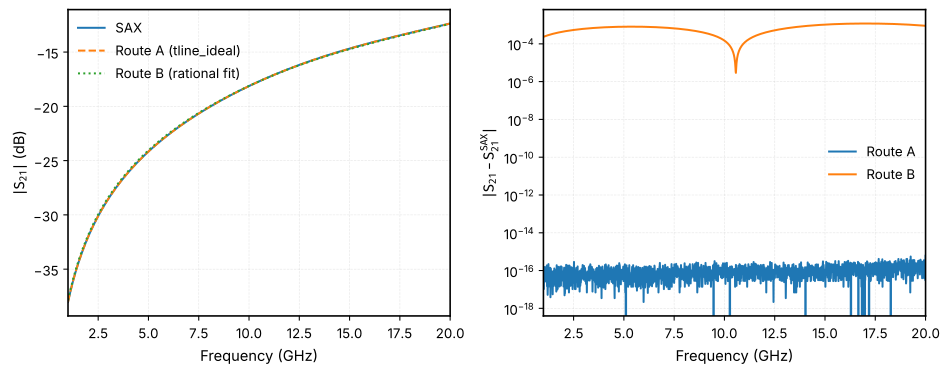
Route A matches SAX to rounding error. Route B differs by about \(10^{-3}\). That is acceptable for linear S-parameters, but not for a high-Q resonator.
Resonance versus flux
The SQUID has \(I_\text{c,tot}=4\) µA. The resonance is the peak of the
reflection group delay, \(\tau=-\text{d}\arg\Gamma/\text{d}\omega\)
Pozar (2012). For a lossless, overcoupled
one-port resonator \(\tau_\text{peak}=4/\kappa\), so the width
\(4/(2\pi\tau_\text{peak})\) is the linewidth only in that case
Göppl et al. (2008). The SAX reference terminates
the coupled-line ABCD matrix with the admittance of
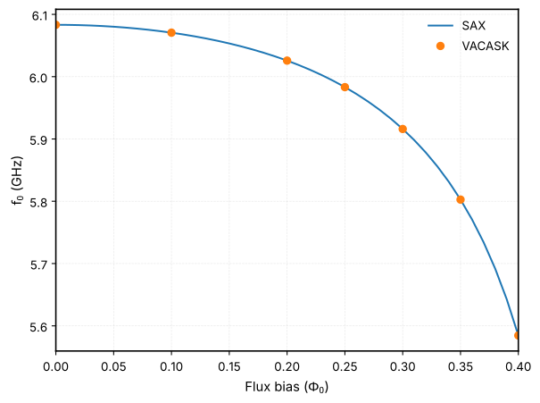
squid_junction Tesche et al. (1977).
AC linearizes the circuit around its DC operating point. With zero pump, it gives the unpumped resonance.
IC_SQUID = 4e-6


def cpw_jpa_netlist(
    control: str,
    *,
    route: str = "A",
    flux: float = 0.3,
    pump: float = 0.0,
    f_pump: float = 1e9,
) -> Netlist:
    """Quarter-wave CPW JPA netlist using Route A or Route B for the line."""
    return Netlist(
        "Quarter-wave CPW JPA",
        loads=[*LINE_LOADS, "squid.va"],
        subckts=[ROUTE_A if route == "A" else ROUTE_B],
        circuit=f"""
            model isource isource
            model vsource vsource
            model resistor resistor
            model capacitor capacitor
            model tline_ideal tline_ideal
            model squid squid

            iin (0 in) isource dc=0 {SMALL_SIGNAL}
            rport (in 0) resistor r={R_PORT}
            x1 (in 2) ccline
            s1 (2 0 fl) squid ic_tot={IC_SQUID}
            vfl (fl 0) vsource type="sine" sinedc={flux} ampl={pump} freq={f_pump}
        """,
        control=f"{OPTIONS}\n{control}",
    )


def resonance(f: jax.Array, gamma: jax.Array) -> tuple[jax.Array, jax.Array]:
    r"""Peak-delay frequency and 4/(2π tau).

    Group delay is $-\text{d}\arg\Gamma/\text{d}\omega$
    :cite:p:`m.pozarMicrowaveEngineering2012`. The second value is a linewidth
    only for a lossless one-port resonator
    :cite:p:`gopplCoplanarWaveguideResonators2008a`.

    Returns:
        Peak-delay frequency and effective delay width, both in Hz.
    """
    grad = jnp.gradient(jnp.unwrap(jnp.angle(gamma)), 2 * jnp.pi * f)
    tau = -jnp.asarray(grad[0] if isinstance(grad, list) else grad)
    k = tau.argmax()
    return f[k], 4 / tau[k] / (2 * jnp.pi)


def sax_reflection(f: jax.Array, flux: float) -> jax.Array:
    """Reflection of the SAX coupled line terminated by the SAX SQUID.

    The SQUID admittance follows :cite:p:`tescheDcSQUIDNoise1977`.

    Returns:
        Complex port reflection coefficients.
    """
    abcd = coupled_line_abcd(f)
    squid = squid_junction(
        f=f, ic_tot=IC_SQUID, capacitance=0.0, resistance=1e12, flux=flux * Φ_0
    )
    # Series element referenced to 50 Ω: S11 = Z / (Z + 2 Z0).
    s11 = squid["o1", "o1"]
    y_load = (1 - s11) / (2 * 50.0 * s11)
    z_in = (abcd[:, 0, 0] / y_load + abcd[:, 0, 1]) / (
        abcd[:, 1, 0] / y_load + abcd[:, 1, 1]
    )
    return (z_in - R_PORT) / (z_in + R_PORT)


fluxes = [0.0, 0.1, 0.2, 0.25, 0.3, 0.35, 0.4]
ac = vacask.run(
    cpw_jpa_netlist(f"""
        sweep flux instance="vfl" parameter="sinedc" values={format_value(fluxes)}
        analysis ac1 ac from=5.4e9 to=6.2e9 mode="lin" points=160001
    """)
)["ac1"]
f_grid = jnp.linspace(5.4e9, 6.2e9, 160001)
f_res = jnp.array(
    [
        resonance(jnp.asarray(g["frequency"].real), reflection(g["in"], I_SIG))[0]
        for g in ac.split("flux")
    ]
)
f_sax = jnp.array(
    [resonance(f_grid, sax_reflection(f_grid, flux))[0] for flux in fluxes]
)
for flux, f0, f0_sax in zip(fluxes, f_res, f_sax, strict=True):
    print(f"Φ = {flux:.2f} Φ0: VACASK {f0 / 1e9:.5f} GHz, SAX {f0_sax / 1e9:.5f} GHz")

fluxes_fine = jnp.linspace(0, 0.4, 41)
f_sax_fine = jnp.array(
    [resonance(f_grid, sax_reflection(f_grid, flux))[0] for flux in fluxes_fine]
)
fig, ax = plt.subplots()
ax.plot(fluxes_fine, f_sax_fine / 1e9, "-", label="SAX")
ax.plot(fluxes, f_res / 1e9, "o", label="VACASK")
ax.set_xlabel(r"Flux bias ($\Phi_0$)")
ax.set_ylabel(r"$f_0$ (GHz)")
ax.legend()
show_plot()
Φ = 0.00 Φ0: VACASK 6.08328 GHz, SAX 6.08328 GHz
Φ = 0.10 Φ0: VACASK 6.07064 GHz, SAX 6.07064 GHz
Φ = 0.20 Φ0: VACASK 6.02580 GHz, SAX 6.02580 GHz
Φ = 0.25 Φ0: VACASK 5.98322 GHz, SAX 5.98322 GHz
Φ = 0.30 Φ0: VACASK 5.91600 GHz, SAX 5.91600 GHz
Φ = 0.35 Φ0: VACASK 5.80267 GHz, SAX 5.80267 GHz
Φ = 0.40 Φ0: VACASK 5.58455 GHz, SAX 5.58455 GHz
Operating point and the single-mode threshold
For \(\omega_0(t)=\omega_0+\delta\omega\cos(2\omega_0t)\), single-mode theory Roy et al. (2016) gives the threshold \(\delta\omega=\kappa\) and the center gain
We measure \(f_0\), \(\kappa\) and \(\text{d}f_0/\text{d}\Phi\) at \(\Phi=0.3\,\Phi_0\) from AC sweeps. These runs have no pump, so the delay gives the unpumped linewidth.
FLUX_BIAS = 0.3
operating_fluxes = [FLUX_BIAS - 1e-3, FLUX_BIAS, FLUX_BIAS + 1e-3]
ac = vacask.run(
    cpw_jpa_netlist(f"""
        sweep flux instance="vfl" parameter="sinedc" values={format_value(operating_fluxes)}
        analysis ac1 ac from=5.85e9 to=6.0e9 mode="lin" points=150001
    """)
)["ac1"]
operating = [
    resonance(jnp.asarray(g["frequency"].real), reflection(g["in"], I_SIG))
    for g in ac.split("flux")
]
(f_lo, _), (F0, KAPPA), (f_hi, _) = (tuple(map(float, x)) for x in operating)
DF_DPHI = (f_hi - f_lo) / 2e-3
PUMP_THRESHOLD = KAPPA / abs(DF_DPHI)
print(f"f0 = {F0 / 1e9:.6f} GHz, κ/2π = {KAPPA / 1e6:.3f} MHz, Q = {F0 / KAPPA:.0f}")
print(f"df0/dΦ = {DF_DPHI / 1e9:.4f} GHz/Φ0")
print(f"single-mode threshold Φp = {PUMP_THRESHOLD:.5f} Φ0")
f0 = 5.916001 GHz, κ/2π = 10.242 MHz, Q = 578
df0/dΦ = -1.7005 GHz/Φ0
single-mode threshold Φp = 0.00602 Φ0
Gain versus pump amplitude
Pump at \(f_\text{p}=2f_0\) below threshold and compare with Eq. (1).
hbac first solves the pump state, then finds the infinitesimal signal and
idler around it. By default it also solves the pump HB, so no separate HB run
is needed. See the Choose a VACASK analysis.
At \(f_\text{s}=f_\text{p}/2\) the signal and idler share one frequency and the gain depends on the signal phase. The sweep skips that point, so each curve is the phase-preserving gain of a slightly detuned signal.
F_PUMP_CPW = 2 * F0
ratios = jnp.array([0.3, 0.5, 0.7, 0.8, 0.9])
# The 1.0013 keeps the 200-point grid off the degenerate point f_s = F0.
plot = vacask.run(
    cpw_jpa_netlist(
        f"""
        sweep pump instance="vfl" parameter="ampl" \\
            values={format_value(ratios * PUMP_THRESHOLD)}
        analysis hbac1 hbac freq=[{F_PUMP_CPW}] nharm=5 outspur={{[0],[-1]}} \\
            from={F0 - 1.0013 * KAPPA} to={F0 + 1.0013 * KAPPA} mode="lin" points=200
        """,
        f_pump=F_PUMP_CPW,
    )
)["hbac1"]

fig, ax = plt.subplots()
for group, r in zip(plot.split("pump"), ratios, strict=True):
    detuning = (jnp.asarray(group["frequency"].real) - F0) / KAPPA
    gain = db(reflection(group["in;0"], I_SIG))
    idler = db(conversion(group["in;-1"], I_SIG))
    k = jnp.argmin(jnp.abs(detuning))
    analytic = 20 * jnp.log10((1 + r**2) / (1 - r**2))
    print(
        f"r = {r:.1f}: peak gain {gain.max():5.2f} dB (single-mode {analytic:5.2f} dB), "
        f"|S_ss|² - |S_is|² = {10 ** (gain[k] / 10) - 10 ** (idler[k] / 10):.3f}"
    )
    (line,) = ax.plot(detuning, gain, label=f"{r:.1f}")
    ax.axhline(float(analytic), color=line.get_color(), ls=":", lw=1)
ax.set_xlabel(r"Signal detuning $(f_\text{s} - f_0)/(\kappa/2\pi)$")
ax.set_ylabel("Signal gain (dB)")
ax.legend(title=r"$\Phi_\text{p}$ / threshold")
ax.set_title("Solid: VACASK hbac; dotted: single-mode peak gain")
show_plot()
r = 0.3: peak gain  1.26 dB (single-mode  1.57 dB), |S_ss|² - |S_is|² = 0.932
r = 0.5: peak gain  3.42 dB (single-mode  4.44 dB), |S_ss|² - |S_is|² = 0.786
r = 0.7: peak gain  6.53 dB (single-mode  9.31 dB), |S_ss|² - |S_is|² = 0.492
r = 0.8: peak gain  8.46 dB (single-mode 13.17 dB), |S_ss|² - |S_is|² = 0.241
r = 0.9: peak gain 10.70 dB (single-mode 19.58 dB), |S_ss|² - |S_is|² = -0.136
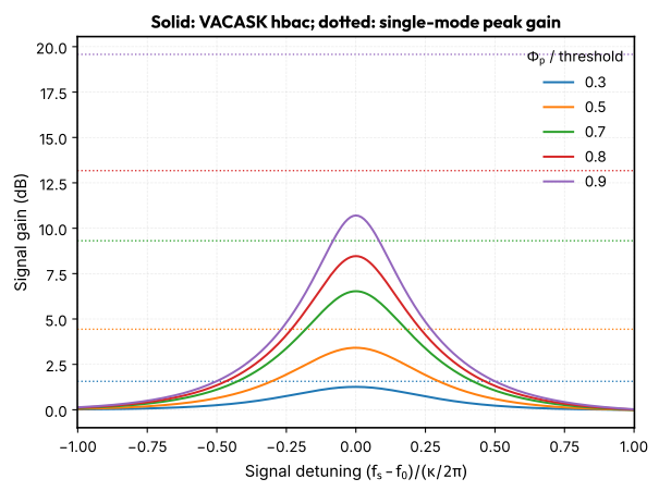
The CPW JPA gives less gain than Eq. (1), and the
two-mode balance \(|S_\text{ss}|^2-|S_\text{is}|^2\) falls below 1. Photons
leave through other sidebands. A quarter-wave line has modes near
\((2n+1)f_0\), spaced by \(2f_0=f_\text{p}\). Every sideband
\(|f_\text{s}+k f_\text{p}|\) then lands near a mode. For \(k=+1\) and \(k=-2\) that
is the \(3\lambda/4\) mode, and for \(k=+2\) and \(k=-3\) the \(5\lambda/4\) mode. The
pump couples the signal to these modes by frequency conversion (\(k>0\)) and by
further amplification (\(k<0\)). The SQUID's lumped inductance shifts the
higher modes slightly away from the odd harmonics, which limits this
conversion without removing it. A single-mode model cannot capture this.
{cite:t}wustmannNondegenerateParametricResonance2017 analyse such intermode
processes.
A lossless pumped circuit conserves photons. That is the Manley-Rowe relation Manley et al. (1956):
Negative-frequency sidebands enter with a minus sign because they are
amplified, not converted Clerk et al. (2010). The next
cell locates the \(3\lambda/4\) mode and evaluates the sum over every sideband
that hbac retains.
ac = vacask.run(
    cpw_jpa_netlist('analysis ac1 ac from=12e9 to=22e9 mode="lin" points=100001')
)["ac1"]
f_ac = jnp.asarray(ac["frequency"].real)
v_mode = jnp.abs(jnp.asarray(ac["2"]))
peaks = jnp.flatnonzero((v_mode[1:-1] > v_mode[:-2]) & (v_mode[1:-1] > v_mode[2:])) + 1
print(
    "modes between 12 and 22 GHz:", ", ".join(f"{f_ac[p] / 1e9:.3f} GHz" for p in peaks)
)
print(f"f_s + f_p at f_s = f_0: {(F0 + F_PUMP_CPW) / 1e9:.3f} GHz")

NHARM = 5
sidebands = list(range(-NHARM, NHARM + 1))
f_signal = F0 + 0.01 * KAPPA
photon_flux = {}
for r in (0.5, 0.9):
    group = vacask.run(
        cpw_jpa_netlist(
            f"""
            analysis hbac1 hbac freq=[{F_PUMP_CPW}] nharm={NHARM} \\
                outspur={format_value([[k] for k in sidebands])} values=[{f_signal}]
            """,
            pump=r * PUMP_THRESHOLD,
            f_pump=F_PUMP_CPW,
        )
    )["hbac1"]
    photons = []
    for k in sidebands:
        f_k = f_signal + k * F_PUMP_CPW
        amplitude = (reflection if k == 0 else conversion)(group[f"in;{k}"][0], I_SIG)
        photons.append(jnp.sign(f_k) * jnp.abs(amplitude) ** 2 * f_signal / abs(f_k))
    photon_flux[r] = jnp.array(photons)
    parts = ", ".join(
        f"{k:+d}: {p:+.4f}"
        for k, p in zip(sidebands, photons, strict=True)
        if abs(p) > 1e-4
    )
    print(f"r = {r}: {parts}; sum = {photon_flux[r].sum():.6f}")

refined = vacask.run(
    cpw_jpa_netlist(
        f"""
        analysis hbac1 hbac freq=[{F_PUMP_CPW}] nharm={NHARM + 4} \\
            outspur={{[0]}} values=[{f_signal}]
        """,
        pump=0.9 * PUMP_THRESHOLD,
        f_pump=F_PUMP_CPW,
    )
)["hbac1"]
basis_change = jnp.abs(
    reflection(refined["in;0"][0], I_SIG) - reflection(group["in;0"][0], I_SIG)
)
print(f"r = 0.9, nharm {NHARM} -> {NHARM + 4}: |ΔS_ss| = {basis_change:.1e}")

fig, (ax_modes, ax_bars) = plt.subplots(1, 2, figsize=(10, 4))
ax_modes.semilogy(f_ac / 1e9, v_mode)
ax_modes.axvline((F0 + F_PUMP_CPW) / 1e9, color="gray", ls=":")
ax_modes.annotate(
    r"$f_0 + f_\text{p}$",
    ((F0 + F_PUMP_CPW) / 1e9, 0.95),
    xycoords=("data", "axes fraction"),
)
ax_modes.set_xlabel("Frequency (GHz)")
ax_modes.set_ylabel(r"$|V_\text{SQUID}|$ for 1 nA drive (V)")
x = jnp.arange(len(sidebands))
for offset, (r, photons) in zip((-0.2, 0.2), photon_flux.items(), strict=True):
    ax_bars.bar(x + offset, photons, width=0.4, label=f"r = {r}")
ax_bars.set_xticks(x, [f"{k:+d}" for k in sidebands])
# |k| > 3 carries under 1e-4 of the flux.
ax_bars.set_xlim(NHARM - 3.6, NHARM + 3.6)
ax_bars.axhline(0, color="black", lw=0.8)
ax_bars.set_xlabel("Sideband $k$")
ax_bars.set_ylabel("Weighted photon flux")
ax_bars.legend()
fig.tight_layout()
show_plot()
modes between 12 and 22 GHz: 17.787 GHz
f_s + f_p at f_s = f_0: 17.748 GHz
r = 0.5: -3: -0.0003, -2: -0.0630, -1: -1.4071, +0: +2.1934, +1: +0.2758, +2: +0.0012; sum = 0.999998
r = 0.9: -3: -0.0250, -2: -1.7248, -1: -11.8197, +0: +11.6938, +1: +2.8344, +2: +0.0412, +3: +0.0001; sum = 0.999997
r = 0.9, nharm 5 -> 9: |ΔS_ss| = 1.3e-10
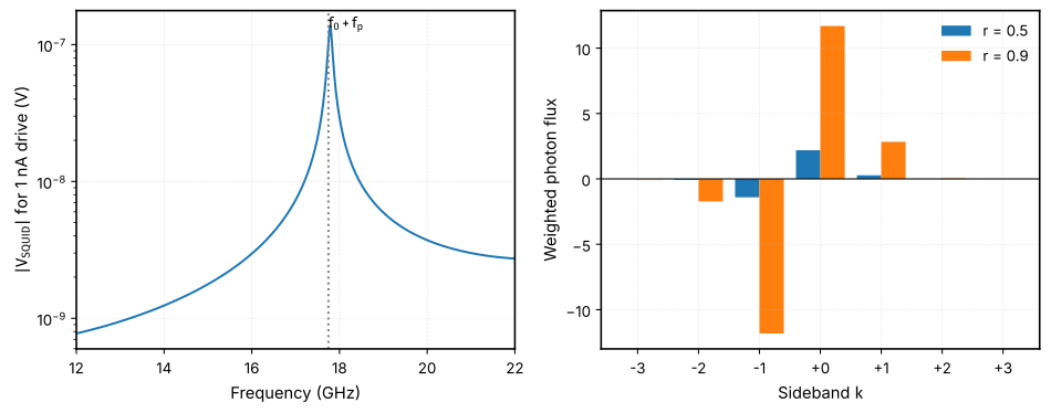
Eq. (2) holds to \(3\times10^{-6}\) at both drives.
At \(r=0.9\) the signal and idler alone would give \(-0.13\). The \(3\lambda/4\)
sidebands \(k=+1\) and \(k=-2\) carry most of the difference, and the
\(5\lambda/4\) sidebands contribute \(+0.041\) (\(k=+2\)) and \(-0.025\) (\(k=-3\)). So the gain lost
relative to Eq. (1) is fully accounted for by intermode
conversion. Raising nharm from 5 to 9 changes the signal reflection by
less than \(10^{-9}\), so the harmonic basis is converged.
Warning
hbaclinearizes around the pumped state whether or not it is stable. Above threshold that state is unstable and the reported gain is not physical.
Route B with the SQUID attached
The rational subcircuit contains only linear elements, so it works in harmonic balance. Its residual fit error appears as loss at the high-Q resonance.
fig, ax = plt.subplots()
for route in "AB":
    ac = vacask.run(
        cpw_jpa_netlist(
            'analysis ac1 ac from=5.85e9 to=6.0e9 mode="lin" points=150001',
            route=route,
        )
    )["ac1"]
    f = jnp.asarray(ac["frequency"].real)
    gamma = reflection(ac["in"], I_SIG)
    f0, delay_width = resonance(f, gamma)
    metric = "κ/2π" if route == "A" else "4/(2π τ_peak)"
    print(
        f"Route {route}: f0 = {f0 / 1e9:.5f} GHz, {metric} = {delay_width / 1e6:.2f} MHz, "
        f"min |Γ| = {jnp.abs(gamma).min():.3f}"
    )
    ax.plot(f / 1e9, jnp.abs(gamma), label=f"Route {route}")
ax.set_xlabel("Frequency (GHz)")
ax.set_ylabel(r"$|\Gamma|$")
ax.legend()
show_plot()
Route A: f0 = 5.91600 GHz, κ/2π = 10.24 MHz, min |Γ| = 1.000
Route B: f0 = 5.91566 GHz, 4/(2π τ_peak) = 9.08 MHz, min |Γ| = 0.463
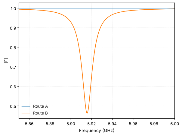
Route B gives min \(|\Gamma|=0.463\) at resonance. Its \(10^{-3}\) S-parameter error introduces appreciable loss in a \(Q\approx580\) resonator. Its \(4/(2\pi\tau_\text{peak})=9.08\) MHz is an effective group-delay quantity, not a loaded linewidth. The lossless identity used for Route A no longer applies. Use Route A, or tighten the fit near resonance, when the line sets amplifier \(Q\).
Limitations
- Classical. HB gives classical gain and conversion. It does not give
added noise or squeezing ({cite:t}
clerkIntroductionQuantumNoise2010; {cite:t}royIntroductionParametricAmplification2016). The junction shunt conductance is noiseless. - Threshold and stability. The single-mode threshold comes from AC scans.
It assumes a purely phase-modulated resonance.
hbaclinearizes around the pumped state whether or not it is stable. Above threshold the reported gain is not physical. - Route B fit loss. A \(10^{-3}\) rational fit adds appreciable loss in this \(Q\approx580\) resonator. Its group delay cannot be read as a lossless linewidth. The fit covers 10 MHz to 70 GHz.
- Multimode gain. Eq. (1) ignores the higher line modes, so it overestimates the gain of this resonator. Its threshold is also only an estimate. A design that needs single-mode behaviour should detune the \(3\lambda/4\) mode from \(3f_0\), for example with a larger SQUID participation or a stepped-impedance line.
- Junction and SQUID models. RCSJ keeps only the first Josephson harmonic McCumber (1968), Tinkham (2015); real junctions show higher ones Willsch et al. (2024). The SQUID model neglects loop inductance and asymmetry.
References
- Yamamoto, T. and Inomata, K. and Watanabe, M. and Matsuba, K. and Miyazaki, T. and Oliver, W. D. and Nakamura, Y. and Tsai, J. S., Flux-Driven Josephson Parametric Amplifier, Applied Physics Letters, 93(4):042510, 2008. doi:10.1063/1.2964182
- Kundert, K.S. and Sangiovanni-Vincentelli, A., Simulation of Nonlinear Circuits in the Frequency Domain, IEEE Transactions on Computer-Aided Design of Integrated Circuits and Systems, 5(4):521–535, 1986. doi:10.1109/TCAD.1986.1270223
- Maas, Stephen A., Nonlinear Microwave and RF Circuits, Artech House, 2003.
- Pozar, David M., Microwave Engineering, John Wiley & Sons, 2012.
- Tesche, Claudia D. and Clarke, John, dc SQUID: Noise and optimization, Journal of Low Temperature Physics, 29(3-4):301–331, 1977. doi:10.1007/BF00655097
- Simons, Rainee N., Coplanar Waveguide Circuits, Components, and Systems, John Wiley & Sons, 2001. doi:10.1002/0471224758
- Ghione, G. and Naldi, C., Analytical Formulas for Coplanar Lines in Hybrid and Monolithic MICs, Electronics Letters, 20(4):179–181, 1984. doi:10.1049/el:19840120
- Gustavsen, B. and Semlyen, A., Rational approximation of frequency domain responses by vector fitting, IEEE Transactions on Power Delivery, 14(3):1052–1061, 1999. doi:10.1109/61.772353
- Göppl, M. and Fragner, A. and Baur, M. and Bianchetti, R. and Filipp, S. and Fink, J. M. and Leek, P. J. and Puebla, G. and Steffen, L. and Wallraff, A., Coplanar Waveguide Resonators for Circuit Quantum Electrodynamics, Journal of Applied Physics, 104(11):113904, 2008. doi:10.1063/1.3010859
- Roy, Ananda and Devoret, Michel, Introduction to Parametric Amplification of Quantum Signals with Josephson Circuits, Comptes Rendus Physique, 17(7):740–755, 2016. doi:10.1016/j.crhy.2016.07.012
- Manley, J. M. and Rowe, H. E., Some General Properties of Nonlinear Elements-Part I. General Energy Relations, Proceedings of the IRE, 44(7):904–913, 1956. doi:10.1109/JRPROC.1956.275145
- Clerk, A. A. and Devoret, M. H. and Girvin, S. M. and Marquardt, Florian and Schoelkopf, R. J., Introduction to Quantum Noise, Measurement, and Amplification, Reviews of Modern Physics, 82(2):1155–1208, 2010. doi:10.1103/RevModPhys.82.1155
- McCumber, D. E., Effect of ac Impedance on dc Voltage-Current Characteristics of Superconductor Weak-Link Junctions, Journal of Applied Physics, 39(7):3113–3118, 1968. doi:10.1063/1.1656743
- Tinkham, Michael, Introduction to Superconductivity, Dover Publ, 2015.
- Willsch, Dennis and Rieger, Dennis and Winkel, Patrick and Willsch, Madita and Dickel, Christian and Krause, Jonas and Ando, Yoichi and Lescanne, Raphaël and Leghtas, Zaki and Bronn, Nicholas T. and Deb, Pratiti and Lanes, Olivia and Minev, Zlatko K. and Dennig, Benedikt and Geisert, Simon and Günzler, Simon and Ihssen, Sören and Paluch, Patrick and Reisinger, Thomas and Hanna, Roudy and Bae, Jin Hee and Schüffelgen, Peter and Grützmacher, Detlev and Buimaga-Iarinca, Luiza and Morari, Cristian and Wernsdorfer, Wolfgang and DiVincenzo, David P. and Michielsen, Kristel and Catelani, Gianluigi and Pop, Ioan M., Observation of Josephson Harmonics in Tunnel Junctions, Nature Physics, 20(5):815–821, 2024. doi:10.1038/s41567-024-02400-8