MZM RF Transmission Line Model (SAX)
The voltage integration method
The following sections describe using the voltage integration method to determine the RF properties of a Mach-Zehnder Modulator (MZM). More information can be found in Pupalaikis2023. The mathematical idea is to discretize the traveling wave modulator and integrate the voltage along the line, accounting for the walk-off between the optical and electrical wave. This is essentially a circuit implementation of the matrix method shown in Li2004.
The generic implementation from a circuit perspective creates the following unit cell:
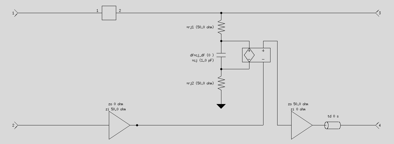
The circuit consists of 3 main sections:
- Unloaded transmission line — abstracted as a 2-port network. This can represent an RLGC element, a unit-cell simulated by FEM, or any other model for the S-parameters of a transmission line segment without lumped elements attached.
- Active diode section — represents the PN junction as an RC network to ground.
- Voltage monitor — the voltage across the capacitor is monitored by a voltage-controlled voltage source (VCVS) connected to a time delay. The time delay represents the optical group delay of the light envelope passing through this unit of the MZM.
By having the electrical signal travel along with the optical signal and being summed each time by the VCVS, the voltage is effectively integrated along the line. The unit cell can be cascaded many times to determine the response of the MZM. This creates an equivalent circuit to the mathematical expression above. The advantage of the circuit approach is that it requires no post-processing and can be extracted directly from circuit analysis.
Upper bound on EO bandwidth from electrical S21
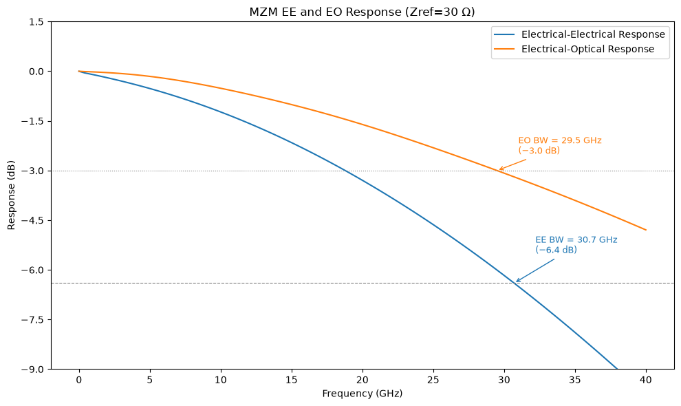
Under perfect velocity and impedance matching between the microwave and optical waves (\(n_\mathrm{opt} = n_\mu\)), the electro-optic 3 dB bandwidth corresponds to a propagation loss condition of \(\alpha l = 0.7384\). At this condition, the electrical insertion loss evaluates to:
This means that under ideal velocity matching, measuring the frequency at which \(|S_{21}|\) drops to \(-6.4\ \mathrm{dB}\) directly yields the EO 3 dB cut-off frequency.
In practice, velocity mismatch introduces additional phase walk-off which reduces modulation efficiency at high frequencies. The EO bandwidth is therefore always lower than the \(-6.4\ \mathrm{dB}\) electrical criterion, making it a theoretical upper bound.
References
- [Pupalaikis2023] Alloin, Laurent & de Valicourt, Guilhem & Pupalaikis, Peter & Elsinger, Lukas & Daunt, Chris. (2023). Simulation and Analysis of Electrical/Optical Communication Links Using OpenSource Software.
- [Li2004] Li et al (2004). Analysis of segmented traveling-wave optical modulators.
Implementation in SAX
import jax
import jax.numpy as jnp
import matplotlib.pyplot as plt
import skrf as rf

jax.config.update("jax_enable_x64", True)
Unloaded transmission line
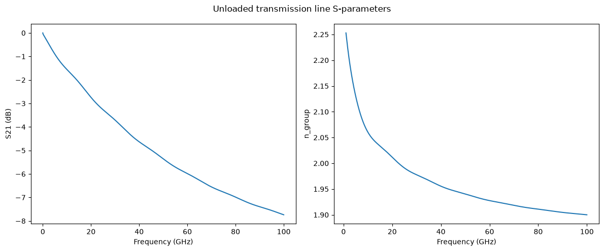
The unloaded transmission line is described using a causal model from Djordjevic and Svensson, ported to JAX for compatibility with SAX's functional style.
from functools import partial

import sax

C0 = 2.99792458e8


def ep_r_djordjevicsvensson(f, ep_r, tanD, f_low=1e3, f_high=1e12, f_ep=1e9):
    """Djordjevic/Svensson wideband Debye dispersion model."""
    k = jnp.log((f_high + 1j * f_ep) / (f_low + 1j * f_ep))
    fd = jnp.log((f_high + 1j * f) / (f_low + 1j * f))
    ep_d = -tanD * ep_r / jnp.imag(k)
    ep_inf = ep_r * (1.0 + tanD * jnp.real(k) / jnp.imag(k))
    return ep_inf + ep_d * fd


def alpha_conductor(f, A, f_A, A0=0.0):
    """Conductor attenuation constant with optional DC resistive loss term."""
    return A0 + A * jnp.log(10) / 20.0 * jnp.sqrt(f / f_A)


def alpha_dielectric(f, ep_r_f):
    """Dielectric attenuation constant."""
    ep_real = jnp.real(ep_r_f)
    tand_f = -jnp.imag(ep_r_f) / ep_real
    return jnp.pi * jnp.sqrt(ep_real) * f / C0 * tand_f


def beta_phase(f, ep_r_f):
    """Phase constant."""
    return 2.0 * jnp.pi * f * jnp.sqrt(jnp.real(ep_r_f)) / C0


def _tline_sparams(f, ep_r_f, A, f_A, z0_char, z0_port, length, A0=0.0):
    """Core S-parameter kernel."""
    alpha_c = alpha_conductor(f, A, f_A, A0)
    alpha_d = alpha_dielectric(f, ep_r_f)
    beta = beta_phase(f, ep_r_f)
    gamma = (alpha_c + alpha_d) + 1j * beta

    gl = gamma * length
    exp_gl = jnp.exp(-gl)
    gamma_r = (z0_char - z0_port) / (z0_char + z0_port)
    denom = 1.0 - gamma_r**2 * jnp.exp(-2 * gl)

    s11 = gamma_r * (1.0 - jnp.exp(-2 * gl)) / denom
    s21 = exp_gl * (1.0 - gamma_r**2) / denom

    return {
        ("o1", "o1"): s11,
        ("o1", "o2"): s21,
        ("o2", "o1"): s21,
        ("o2", "o2"): s11,
    }


def tline_ds(
    *,
    frequency=1e9,
    length=1e-3,
    A=0.0,
    f_A=1.0,
    ep_r=1.0,
    tanD=0.0,
    z0_characteristic=50.0,
    z0=50.0,
    f_low=1e3,
    f_high=1e12,
    f_ep=1e9,
):
    """SAX 2-port S-parameter model with Djordjevic/Svensson dispersive dielectric."""
    ep_r_f = ep_r_djordjevicsvensson(frequency, ep_r, tanD, f_low, f_high, f_ep)
    return _tline_sparams(
        frequency,
        ep_r_f,
        A,
        f_A,
        z0_char=z0_characteristic,
        z0_port=z0,
        length=length,
    )


unloaded_model = partial(tline_ds, f_low=1e9, f_high=100e9, f_ep=20e9)


def half_tline_ds(
    *,
    frequency=1e9,
    length=1e-3,
    A=0.0,
    f_A=1.0,
    ep_r=1.0,
    tanD=0.0,
    z0_characteristic=85.0,
    z0=50.0,
):
    """Half-length transmission line for the loaded unit cell."""
    return unloaded_model(
        frequency=frequency,
        length=0.5 * length,
        A=A,
        f_A=f_A,
        ep_r=ep_r,
        tanD=tanD,
        z0_characteristic=z0_characteristic,
        z0=z0,
    )
length = 5000e-6
tline_params = {
    "ep_r": 4.04,
    "tanD": 0.11,
    "A": 0.0009,
    "z0_characteristic": 60.0,
    "z0": 50,
    "f_low": 1e9,
    "f_high": 100e9,
    "f_ep": 20e9,
}

multiplier = 1e9
f = jnp.arange(1e-6, 100, 1e-2)

s = tline_ds(frequency=f * multiplier, length=length, **tline_params)

fig, axes = plt.subplots(ncols=2, figsize=(12, 5))
axes[0].plot(f, rf.complex_2_db(s["o2", "o1"]))
axes[0].set_xlabel("Frequency (GHz)")
axes[0].set_ylabel("S21 (dB)")

ng = (
    -C0
    * rf.unwrap(rf.complex_2_radian(s["o2", "o1"]))
    / (length * 2.0 * jnp.pi * f * multiplier)
)
axes[1].plot(f[100:], ng[100:])
axes[1].set_xlabel("Frequency (GHz)")
axes[1].set_ylabel("n_group")
plt.suptitle("Unloaded transmission line S-parameters")
plt.tight_layout()
/tmp/ipykernel_3367/2296271145.py:19: FutureWarning: skrf.complex_2_db is deprecated. Please import complex_2_db from skrf.mathFunctions instead.
  axes[0].plot(f, rf.complex_2_db(s["o2", "o1"]))
/tmp/ipykernel_3367/2296271145.py:25: FutureWarning: skrf.complex_2_radian is deprecated. Please import complex_2_radian from skrf.mathFunctions instead.
  * rf.unwrap(rf.complex_2_radian(s["o2", "o1"]))
Additional devices
Several additional devices are needed to integrate the voltage along the line:
- Voltage-controlled voltage source (VCVS)
- Optical group delay line
- 2-port voltage amplifier
- Series resistor / capacitor (per-length variants)
- Splitter (n-port tee)
- Ground termination
from sax.constants import C_M_S


def vcvs(*, gain=1.0):
    """Voltage-controlled voltage source (4-port)."""
    one = 1.0
    return sax.sdict(
        {
            ("o1", "o1"): one,
            ("o2", "o2"): one,
            ("o3", "o1"): gain * one,
            ("o3", "o2"): -gain * one,
            ("o3", "o4"): one,
            ("o4", "o1"): -gain * one,
            ("o4", "o2"): gain * one,
            ("o4", "o3"): one,
        }
    )


def delay_line(*, frequency=1e9, time_delay=2e-15, zc=50.0, z0_port=50.0):
    """Lossless transmission line delay (2-port)."""
    w = 2.0 * jnp.pi * frequency
    gamma = 1j * w * time_delay
    p = (zc - z0_port) / (zc + z0_port)
    prop = jnp.exp(-gamma)
    denom = 1.0 - (p * prop) ** 2
    S11 = p * (1.0 - prop**2) / denom
    S21 = (1.0 - p**2) * prop / denom
    return sax.reciprocal({("o1", "o1"): S11, ("o1", "o2"): S21, ("o2", "o2"): S11})


def optical_group_delay(*, frequency=5e9, length=1.0, ng=4.05, zc=50, z0_port=50):
    """Delay line parameterized by optical group index and physical length."""
    return delay_line(
        zc=zc, z0_port=z0_port, frequency=frequency, time_delay=length * ng / C_M_S
    )


def voltage_amplifier_two_port(g=1.0, zi=50.0, zo=50.0, z0=50.0):
    """Two-port voltage amplifier S-parameters."""
    return {
        ("o1", "o1"): (zi - z0) / (zi + z0),
        ("o2", "o1"): 2.0 * g * zi * z0 / ((zi + z0) * (zo + z0)),
        ("o2", "o2"): (zo - z0) / (zo + z0),
    }


def splitter_factory(num_ports=3):
    """Returns a SAX component for a general n-port lossless splitter/tee."""
    p = num_ports
    ports = [f"o{i + 1}" for i in range(p)]
    eye = jnp.eye(p)

    def splitter(*, z0=50.0):
        z0_arr = jnp.broadcast_to(jnp.asarray(z0, dtype=complex), (p,))
        inv_sum = jnp.sum(1.0 / z0_arr)
        off = (
            2.0
            * jnp.sqrt(jnp.outer(z0_arr.real, z0_arr.real))
            / (jnp.outer(z0_arr, z0_arr) * inv_sum)
        )
        z_load = 1.0 / (inv_sum - 1.0 / z0_arr)
        diag_vals = (z_load - z0_arr.conj()) / (z_load + z0_arr)
        mat = off * (1.0 - eye) + diag_vals[:, None] * eye
        return {
            (pi, pj): mat[i, j]
            for i, pi in enumerate(ports)
            for j, pj in enumerate(ports)
        }

    return splitter


def resistor(*, r, z0=50.0):
    """S-parameters for a series resistor."""
    z0_arr = jnp.broadcast_to(jnp.asarray(z0, dtype=complex), (2,))
    z0_0, z0_1 = z0_arr[0], z0_arr[1]
    r = jnp.asarray(r, dtype=complex)
    denom = r + (z0_0 + z0_1)
    off = 2.0 * jnp.sqrt(z0_0.real * z0_1.real) / denom
    return {
        ("o1", "o1"): (r - z0_0.conj() + z0_1) / denom,
        ("o1", "o2"): off,
        ("o2", "o1"): off,
        ("o2", "o2"): (r + z0_0 - z0_1.conj()) / denom,
    }


def capacitor(*, frequency=1e9, c, z0=50.0):
    """S-parameters for a series capacitor."""
    z0_arr = jnp.broadcast_to(jnp.asarray(z0, dtype=complex), (2,))
    z0_0, z0_1 = z0_arr[0], z0_arr[1]
    w = 2.0 * jnp.pi * jnp.asarray(frequency)
    c = jnp.asarray(c)
    denom = 1.0 + 1j * w * c * (z0_0 + z0_1)
    off = 2j * w * c * jnp.sqrt(z0_0.real * z0_1.real) / denom
    return {
        ("o1", "o1"): (1.0 - 1j * w * c * (z0_0.conj() - z0_1)) / denom,
        ("o1", "o2"): off,
        ("o2", "o1"): off,
        ("o2", "o2"): (1.0 - 1j * w * c * (z0_1.conj() - z0_0)) / denom,
    }


def resistance_length(*, length=1.0, resistance_per_length=4.7e-3, z0=50.0):
    """Series resistor scaled by physical length."""
    return resistor(r=resistance_per_length / length, z0=z0)


def capacitor_per_length(
    *, frequency=5e9, length=1.0, capacitance_per_length=320e-12, z0=50.0
):
    """Series capacitor scaled by physical length."""
    return capacitor(frequency=frequency, c=capacitance_per_length * length, z0=z0)


def gnd():
    """Ground (short-circuit) termination."""
    return {("o1", "o1"): -1.0 + 0j}
Assembling the loaded unit cell
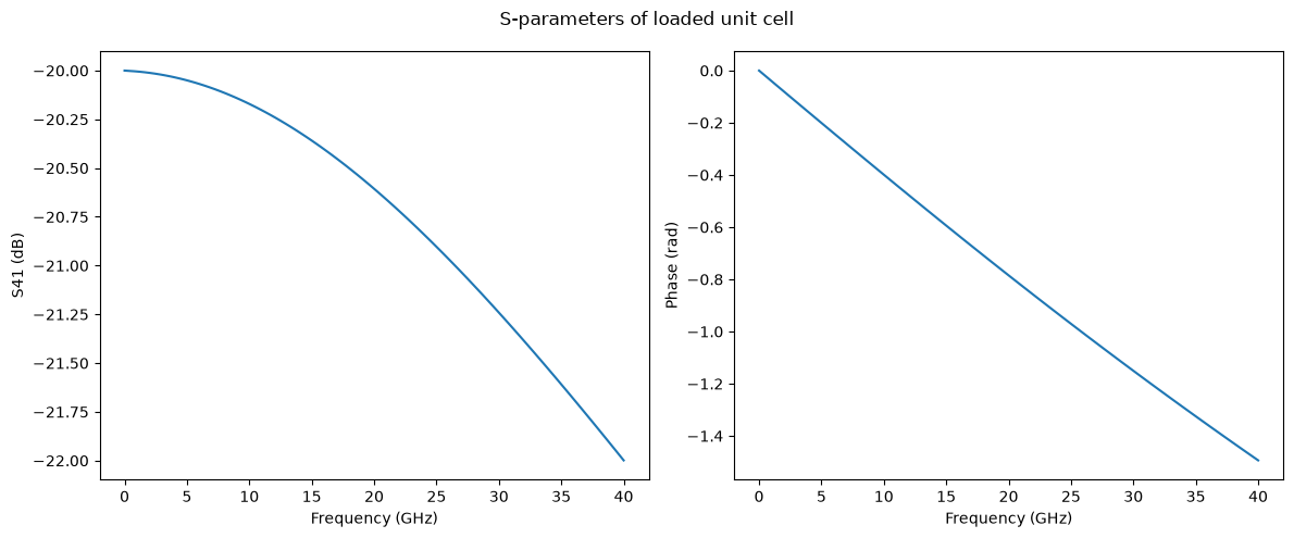
Now that all components are defined, the unit cell can be assembled. Once a unit cell is defined, it is just a matter of cascading the S-parameters to determine the total MZM response.
tline_params = {
    "ep_r": 4.04,
    "tanD": 0.11,
    "A": 0.0009,
    "z0_characteristic": 60,
    "f_low": 1e9,
    "f_high": 100e9,
    "f_ep": 20e9,
}

_loaded_netlist = {
    "instances": {
        "unloaded_in": {"component": "half_tline", "settings": tline_params},
        "unloaded_out": {"component": "half_tline", "settings": tline_params},
        "res1": {"component": "sheet_resistor"},
        "cap1": {"component": "sheet_capacitor"},
        "vcvs1": {"component": "vcvs", "settings": {"gain": 0.1}},
        "delay1": {"component": "delay_line", "settings": {"ng": 4.05}},
        "amp_in": {"component": "amp", "settings": {"g": 1.0, "zi": 50.0, "zo": 0.0}},
        "amp_out": {
            "component": "amp",
            "settings": {"g": 2.0, "zi": 50.0, "zo": 50.0},
        },
        "gnd": {"component": "gnd"},
        "tee_a": {"component": "tee"},
        "tee_b": {"component": "tee"},
        "tee_c": {"component": "tee"},
    },
    "connections": {
        "unloaded_in,o2": "tee_a,o1",
        "unloaded_out,o1": "tee_a,o2",
        "res1,o1": "tee_a,o3",
        "res1,o2": "tee_b,o1",
        "cap1,o1": "tee_b,o2",
        "vcvs1,o2": "tee_b,o3",
        "cap1,o2": "tee_c,o1",
        "vcvs1,o1": "tee_c,o2",
        "gnd,o1": "tee_c,o3",
        "vcvs1,o3": "amp_in,o2",
        "vcvs1,o4": "delay1,o1",
        "delay1,o2": "amp_out,o1",
    },
    "ports": {
        "port0": "unloaded_in,o1",
        "port1": "unloaded_out,o2",
        "port2": "amp_in,o1",
        "port3": "amp_out,o2",
    },
}

loaded_circuit, _ = sax.circuit(
    netlist=_loaded_netlist,
    models={
        "half_tline": half_tline_ds,
        "sheet_resistor": resistance_length,
        "sheet_capacitor": capacitor_per_length,
        "vcvs": vcvs,
        "delay_line": optical_group_delay,
        "amp": voltage_amplifier_two_port,
        "gnd": gnd,
        "tee": splitter_factory(num_ports=3),
    },
)

multiplier = 1e-9
f = jnp.linspace(1e-3, 40, 100) / multiplier

s = loaded_circuit(frequency=f, z0=50, length=200e-6)

fig, axes = plt.subplots(ncols=2, figsize=(12, 5))
axes[0].plot(f * multiplier, rf.complex_2_db(s[("port3", "port0")]))
axes[0].set_xlabel("Frequency (GHz)")
axes[0].set_ylabel("S41 (dB)")
axes[1].plot(f * multiplier, rf.unwrap_rad(rf.complex_2_radian(s[("port3", "port0")])))
axes[1].set_xlabel("Frequency (GHz)")
axes[1].set_ylabel("Phase (rad)")
plt.suptitle("S-parameters of loaded unit cell")
plt.tight_layout()
/tmp/ipykernel_3367/4103021807.py:71: FutureWarning: skrf.complex_2_db is deprecated. Please import complex_2_db from skrf.mathFunctions instead.
  axes[0].plot(f * multiplier, rf.complex_2_db(s[("port3", "port0")]))
/tmp/ipykernel_3367/4103021807.py:74: FutureWarning: skrf.unwrap_rad is deprecated. Please import unwrap_rad from skrf.mathFunctions instead.
  axes[1].plot(f * multiplier, rf.unwrap_rad(rf.complex_2_radian(s[("port3", "port0")])))
/tmp/ipykernel_3367/4103021807.py:74: FutureWarning: skrf.complex_2_radian is deprecated. Please import complex_2_radian from skrf.mathFunctions instead.
  axes[1].plot(f * multiplier, rf.unwrap_rad(rf.complex_2_radian(s[("port3", "port0")])))
Cascading the unit cell
The unit cell is cascaded N times to model the full MZM length. A utility function builds the cascaded SAX circuit by connecting the RF and EO ports of adjacent cells.
def cascade_circuit(*, n_sections, subcircuit, port_connections):
    """Cascade n_sections copies of a SAX circuit by connecting specified ports."""
    instances = {f"cell_{i}": {"component": "cell"} for i in range(n_sections)}
    connections = {
        f"cell_{i},{out_port}": f"cell_{i + 1},{in_port}"
        for i in range(n_sections - 1)
        for out_port, in_port in port_connections.items()
    }
    ports = {
        **{in_port: f"cell_0,{in_port}" for in_port in port_connections.values()},
        **{
            out_port: f"cell_{n_sections - 1},{out_port}"
            for out_port in port_connections
        },
    }
    cascaded, _ = sax.circuit(
        netlist={"instances": instances, "connections": connections, "ports": ports},
        models={"cell": subcircuit},
    )
    return cascaded


def renormalize_s(s, z_old=50.0, z_new=25.0):
    """Renormalize an SDict from z_old to z_new reference impedance."""
    ports = list(dict.fromkeys(pair[0] for pair in s))
    n = len(ports)

    def _to_array(z):
        if isinstance(z, dict):
            return jnp.array([z[p] for p in ports], dtype=float)
        return jnp.broadcast_to(jnp.asarray(z, dtype=float), (n,))

    mat = jnp.moveaxis(
        jnp.stack([jnp.stack([s[(p_out, p_in)] for p_in in ports]) for p_out in ports]),
        [0, 1],
        [-2, -1],
    )
    z_old_arr = _to_array(z_old)
    z_new_arr = _to_array(z_new)
    gamma = (z_new_arr - z_old_arr) / (z_new_arr + z_old_arr)
    Gamma = jnp.diag(gamma)
    eye = jnp.eye(n)
    a = mat - Gamma
    b = eye - Gamma @ mat
    mat_new = jnp.linalg.solve(b.swapaxes(-1, -2), a.swapaxes(-1, -2)).swapaxes(-1, -2)
    return {
        (p_out, p_in): mat_new[..., i, j]
        for i, p_out in enumerate(ports)
        for j, p_in in enumerate(ports)
    }


z0 = 50
zref = 30
n_sections = 10
total_length = 2e-3
unit_length = total_length / n_sections

cascaded_circuit = cascade_circuit(
    n_sections=n_sections,
    subcircuit=loaded_circuit,
    port_connections={"port1": "port0", "port3": "port2"},
)

mzm_circuit, _ = sax.circuit(
    netlist={
        "instances": {
            "cascaded": {"component": "cascaded_circuit"},
            "amp": {"component": "amp", "settings": {"g": 1, "zi": 50, "zo": 0.0}},
        },
        "connections": {"cascaded,port3": "amp,o1"},
        "ports": {
            "port0": "cascaded,port0",
            "port1": "cascaded,port1",
            "port2": "cascaded,port2",
            "port3": "amp,o2",
        },
    },
    models={"cascaded_circuit": cascaded_circuit, "amp": voltage_amplifier_two_port},
)

s_cascade = mzm_circuit(frequency=f, gain=0.1, z0=z0, length=unit_length)
s_cascade = renormalize_s(s_cascade, z_old=z0, z_new=zref)
f_ghz = f * multiplier
ee_response = rf.complex_2_db(s_cascade[("port1", "port0")])
eo_response = rf.complex_2_db(s_cascade[("port3", "port0")])


def crossing_freq(f, response, threshold):
    """Linear interpolation of the first downward threshold crossing."""
    diff = response - threshold
    idx = jnp.where(jnp.diff(jnp.sign(diff)))[0]
    if len(idx) == 0:
        return jnp.nan
    i = idx[0]
    t = -diff[i] / (diff[i + 1] - diff[i])
    return f[i] + t * (f[i + 1] - f[i])


f_ee = crossing_freq(f_ghz, ee_response, -6.4)
f_eo = crossing_freq(f_ghz, eo_response, -3.0)

fig, ax = plt.subplots(figsize=(10, 6))
ax.plot(f_ghz, ee_response, label="Electrical-Electrical Response")
ax.plot(f_ghz, eo_response, label="Electrical-Optical Response")

ax.axhline(y=-6.4, linestyle="--", color="gray", linewidth=0.8)
ax.axhline(y=-3.0, linestyle=":", color="gray", linewidth=0.8)

ax.annotate(
    f"EE BW = {f_ee:.1f} GHz\n($-$6.4 dB)",
    xy=(f_ee, -6.4),
    xytext=(f_ee + 1.5, -5.5),
    arrowprops={"arrowstyle": "->", "color": "C0"},
    color="C0",
    fontsize=9,
)
ax.annotate(
    f"EO BW = {f_eo:.1f} GHz\n($-$3.0 dB)",
    xy=(f_eo, -3.0),
    xytext=(f_eo + 1.5, -2.5),
    arrowprops={"arrowstyle": "->", "color": "C1"},
    color="C1",
    fontsize=9,
)

ax.legend()
ax.set_ylim(-9, 1.5)
ax.set_yticks(jnp.arange(-9, 3.0, 1.5))
ax.set_xlabel("Frequency (GHz)")
ax.set_ylabel("Response (dB)")
ax.set_title(f"MZM EE and EO Response (Zref={zref} Ω)")
plt.tight_layout()
/tmp/ipykernel_3367/1814957602.py:2: FutureWarning: skrf.complex_2_db is deprecated. Please import complex_2_db from skrf.mathFunctions instead.
  ee_response = rf.complex_2_db(s_cascade[("port1", "port0")])
/tmp/ipykernel_3367/1814957602.py:3: FutureWarning: skrf.complex_2_db is deprecated. Please import complex_2_db from skrf.mathFunctions instead.
  eo_response = rf.complex_2_db(s_cascade[("port3", "port0")])