Resonator frequency estimation models
Required extras
This notebook needs the
modelsextra:uv add "qpdk[models]" # or, from a checkout of this repository: uv sync --extra models # or with pip: pip install "qpdk[models]"See the extras reference for what each extra installs.
This example estimates resonance frequencies of superconducting microwave resonators with JAX.
Show code
# Config: filepaths, PDK activation, package imports and simulation target handling
from functools import partial

import jax
import jax.numpy as jnp
import matplotlib.pyplot as plt
import optax
import sax
from tqdm.auto import trange

from qpdk import PDK, logger
from qpdk.models.cpw import cpw_parameters

PDK.activate()

from qpdk.models.resonator import (
    quarter_wave_resonator_coupled,
    resonator_frequency,
)
from qpdk.tech import coplanar_waveguide
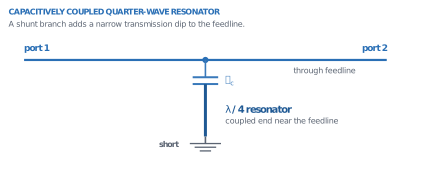
Probelines weakly coupled to \(\lambda/4\) resonator
Creates a probeline weakly coupled to a quarter-wave resonator.
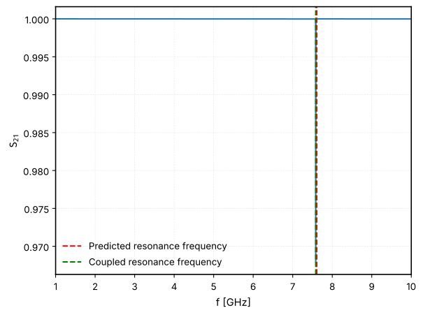
We first estimate the resonance frequency with the resonator_frequency function and then compare it with the resonance of the coupled circuit.
ep_eff, z0 = cpw_parameters(width=10, gap=6)
logger.info(f"{ep_eff=!r}")
logger.info(f"{z0=!r}")  # Characteristic impedance

res_freq = resonator_frequency(
    length=4000,
    epsilon_eff=float(jnp.real(ep_eff)),
    is_quarter_wave=True,
)
logger.info(f"Resonance frequency (quarter-wave): {res_freq / 1e9} GHz")

circuit, _ = sax.circuit(
    netlist={
        "instances": {
            "R1": "quarter_wave_resonator",
        },
        "connections": {},
        "ports": {
            "in": "R1,coupling_o1",
            "out": "R1,coupling_o2",
        },
    },
    models={
        "quarter_wave_resonator": partial(
            quarter_wave_resonator_coupled,
            cross_section=coplanar_waveguide(width=10, gap=6),
        )
    },
)

frequencies = jnp.linspace(1e9, 10e9, 5001)
S = circuit(f=frequencies, length=4000.0)
plt.plot(frequencies / 1e9, abs(S["in", "out"]) ** 2)
plt.xlabel("f [GHz]")
plt.ylabel("$S_{21}$")


def _mark_resonance_frequency(x_value: float | jax.Array, color: str, label: str):
    """Draws a vertical dashed line on the current matplotlib plot to mark a resonance frequency.

    Args:
        x_value: Resonance frequency in Hz. This value is converted to GHz for plotting.
        color: Matplotlib-compatible color specification for the vertical line.
        label: Text label to use in the plot legend for this resonance marker.
    """
    plt.axvline(
        float(x_value) / 1e9,  # Convert frequency from Hz to GHz for plotting
        color=color,
        linestyle="--",
        label=label,
    )


_mark_resonance_frequency(res_freq, "red", "Predicted resonance frequency")
actual_freq = frequencies[jnp.argmin(abs(S["in", "out"]))]
logger.info(f"Coupled resonance frequency: {float(actual_freq) / 1e9} GHz")
_mark_resonance_frequency(actual_freq, "green", "Coupled resonance frequency")

plt.legend()
plt.show()
2026-11-11 05:32:50.184 | INFO     | __main__:<module>:2 - ep_eff=Array(6.06519124-1.49847261e-05j, dtype=complex128)
2026-11-11 05:32:50.185 | INFO     | __main__:<module>:3 - z0=Array(49.31279884, dtype=float64)
2026-11-11 05:32:50.256 | INFO     | __main__:<module>:10 - Resonance frequency (quarter-wave): 7.6081395616176914 GHz
2026-11-11 05:32:57.217 | INFO     | __main__:<module>:56 - Coupled resonance frequency: 7.5826 GHz
Optimizer for given resonance frequency
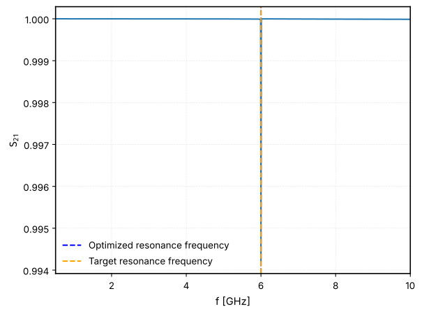
Find the resonator length that gives a desired resonance frequency using an optimizer. Here we use Optax and JAX's automatic differentiation. Instead of evaluating the entire frequency band in every iteration, we minimize the transmission \(|S_{21}|^2\) at the target frequency only. JAX computes the analytical gradient of the transmission with respect to the resonator length, which makes the optimization fast and precise.
TARGET_FREQUENCY = 6e9  # Target resonance frequency in Hz


@jax.jit
def loss_fn(params: dict[str, jnp.ndarray]) -> jnp.ndarray:
    """Loss function to minimize the S21 transmission at the target frequency.

    Args:
        params: Dictionary containing the resonator length in micrometers.

    Returns:
        The loss value as a JAX array.
    """
    length = params["length"]
    # Setup model using the Jittable `circuit` function
    S = circuit(f=jnp.array([TARGET_FREQUENCY]), length=length)
    # S is evaluated at TARGET_FREQUENCY
    # Minimize S21 magnitude at the target frequency
    s21 = S["in", "out"][0]
    return jnp.real(s21 * jnp.conj(s21))


# Test loss function
logger.info(f"Loss at 4000 um: {float(loss_fn({'length': jnp.array(4000.0)}))}")
logger.info(f"Loss at 5900 um: {float(loss_fn({'length': jnp.array(5900.0)}))}")

# To ensure we start within the narrow resonance dip, we first evaluate a coarse array of lengths
expected_length = 4000.0 * (res_freq / TARGET_FREQUENCY)
coarse_lengths = jnp.linspace(expected_length - 1000, expected_length + 1000, 2001)


@jax.jit
@jax.vmap
def sweep_loss(length_val: jnp.ndarray) -> jnp.ndarray:
    """Evaluate loss over a single length value during the initial vmap sweep.

    Args:
        length_val: The length of the resonator in micrometers.

    Returns:
        The loss value for the given length.
    """
    return loss_fn({"length": length_val})


coarse_losses = sweep_loss(coarse_lengths)
best_initial_length = float(coarse_lengths[jnp.argmin(coarse_losses)])
logger.info(f"Best initial guess from sweep: {best_initial_length:.2f} µm")

# Initialize optimizer
params = {"length": jnp.array(best_initial_length)}
optimizer = optax.adam(learning_rate=0.1)
opt_state = optimizer.init(params)


@jax.jit
def step(params, opt_state):
    """Perform a single Optax optimization step to update parameters.

    Args:
        params: Dictionary containing current parameters (e.g., 'length').
        opt_state: Current state of the optimizer.

    Returns:
        A tuple containing (updated parameters, updated opt_state).
    """
    loss_value, grads = jax.value_and_grad(loss_fn)(params)
    updates, opt_state = optimizer.update(grads, opt_state, params)
    params = optax.apply_updates(params, updates)
    return params, opt_state, loss_value


for _ in trange(100, desc="Optimizing"):
    params, opt_state, loss_value = step(params, opt_state)

length_val = float(jax.device_get(params["length"]))
logger.info(f"Optimized Length: {length_val:.2f} µm")

# Evaluate over a range of frequencies to verify
verification_frequencies = jnp.linspace(0.5e9, 10e9, 1001)
optimal_S = circuit(f=verification_frequencies, length=params["length"])
optimal_freq = verification_frequencies[jnp.argmin(abs(optimal_S["in", "out"]))]
optimal_freq_val = float(jax.device_get(optimal_freq))
logger.info(f"Achieved Resonance Frequency: {optimal_freq_val / 1e9:.2f} GHz")

# Plot
plt.close()
plt.plot(verification_frequencies / 1e9, abs(optimal_S["in", "out"]) ** 2)
plt.xlabel("f [GHz]")
plt.ylabel("$S_{21}$")
_mark_resonance_frequency(optimal_freq_val, "blue", "Optimized resonance frequency")
_mark_resonance_frequency(TARGET_FREQUENCY, "orange", "Target resonance frequency")
plt.legend()
plt.show()
2026-11-11 05:33:00.428 | INFO     | __main__:<module>:24 - Loss at 4000 um: 0.9999955174879595
2026-11-11 05:33:00.430 | INFO     | __main__:<module>:25 - Loss at 5900 um: 0.9999957491109099
2026-11-11 05:33:04.004 | INFO     | __main__:<module>:48 - Best initial guess from sweep: 5059.09 µm
2026-11-11 05:33:15.297 | INFO     | __main__:<module>:77 - Optimized Length: 5058.83 µm
2026-11-11 05:33:18.029 | INFO     | __main__:<module>:84 - Achieved Resonance Frequency: 6.00 GHz