Circuit Simulation with QPDK
Required extras
This notebook needs the
modelsextra:uv add "qpdk[models]" # or, from a checkout of this repository: uv sync --extra models # or with pip: pip install "qpdk[models]"See the extras reference for what each extra installs.
This notebook simulates circuits with the qpdk models and the sax circuit solver: first individual components, then a custom resonator circuit built from them.
Show code
# Config: filepaths, PDK activation, package imports and simulation target handling
import jax.numpy as jnp
import sax
from matplotlib import pyplot as plt

from qpdk import PDK
from qpdk.models.generic import capacitor, inductor, tee
from qpdk.models.resonator import quarter_wave_resonator_coupled
from qpdk.models.waveguides import straight, straight_shorted
from qpdk.tech import coplanar_waveguide

PDK.activate()
Setup
First, let's define a frequency range for our simulations and create a coplanar waveguide (CPW) media that defines the transmission line properties.
# Define frequency range
freq = jnp.linspace(2e9, 8e9, 501)
freq_ghz = freq / 1e9

# Define CPW media
cross_section = coplanar_waveguide(width=10, gap=6)
Individual Component Models
Let's simulate some of the basic components available in qpdk.
Straight Waveguide
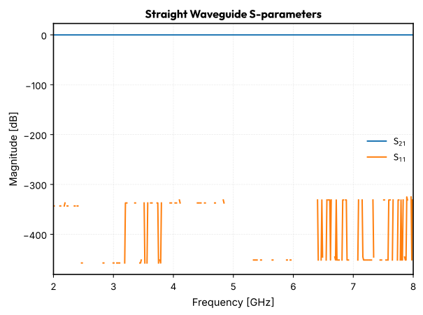
Simulate a \(1\,\text{mm}\) straight waveguide
straight_wg = straight(f=freq, length=1000, cross_section=cross_section)

# Plot S-parameters
plt.figure()
plt.title("Straight Waveguide S-parameters")
plt.plot(freq_ghz, 20 * jnp.log10(jnp.abs(straight_wg["o1", "o2"])), label="$S_{21}$")
plt.plot(freq_ghz, 20 * jnp.log10(jnp.abs(straight_wg["o1", "o1"])), label="$S_{11}$")
plt.xlabel("Frequency [GHz]")
plt.ylabel("Magnitude [dB]")
plt.grid(True)
plt.legend()
plt.show()
Capacitor
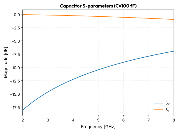
Simulate a \(100\,\text{fF}\) capacitor
cap_val = 100e-15
cap = capacitor(f=freq, capacitance=cap_val, z0=50)

# Plot S-parameters
plt.figure()
plt.title(f"Capacitor S-parameters (C={cap_val * 1e15:.0f} fF)")
plt.plot(freq_ghz, 20 * jnp.log10(jnp.abs(cap["o1", "o2"])), label="$S_{21}$")
plt.plot(freq_ghz, 20 * jnp.log10(jnp.abs(cap["o1", "o1"])), label="$S_{11}$")
plt.xlabel("Frequency [GHz]")
plt.ylabel("Magnitude [dB]")
plt.grid(True)
plt.legend()
plt.show()
Inductor
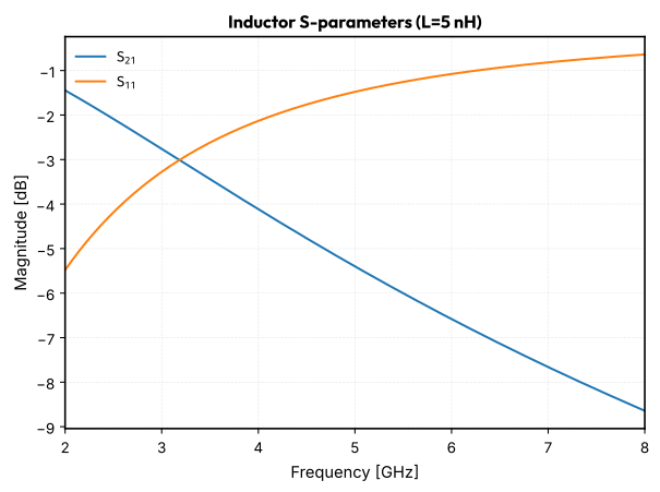
Simulate a \(5\,\text{nH}\) inductor
ind_val = 5e-9
ind = inductor(f=freq, inductance=ind_val, z0=50)

# Plot S-parameters
plt.figure()
plt.title(f"Inductor S-parameters (L={ind_val * 1e9:.0f} nH)")
plt.plot(freq_ghz, 20 * jnp.log10(jnp.abs(ind["o1", "o2"])), label="$S_{21}$")
plt.plot(freq_ghz, 20 * jnp.log10(jnp.abs(ind["o1", "o1"])), label="$S_{11}$")
plt.xlabel("Frequency [GHz]")
plt.ylabel("Magnitude [dB]")
plt.grid(True)
plt.legend()
plt.show()
Coupled Resonator Model
Now let's use a more complex, pre-built model for a coupled resonator.
# Simulate a coupled resonator
res = quarter_wave_resonator_coupled(
    f=freq,
    cross_section=cross_section,
    coupling_gap=0.3,
    coupling_straight_length=200,
    length=5000,
)

# Plot S-parameters
plt.figure()
plt.title("Coupled Resonator S-parameters")
plt.plot(
    freq_ghz,
    20 * jnp.log10(jnp.abs(res["coupling_o1", "coupling_o2"])),
    label="$S_{21}$",
)
plt.xlabel("Frequency [GHz]")
plt.ylabel("Magnitude [dB]")
plt.grid(True)
plt.legend()
plt.show()
Building a Custom Resonator Circuit
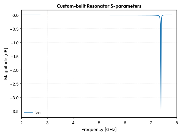
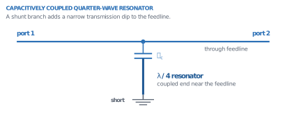
We can use sax to build our own circuits from basic components. Let's build a quarter-wave resonator capacitively coupled to a feedline.
The circuit is a feedline with a T-junction. A capacitor in series with a shorted transmission line (the resonator) connects to the T-junction as a shunt element.
# Define component settings
feedline_segment_length = 500  # um
resonator_length = 4000  # um
coupling_cap_val = 20e-15  # F

# Define models for sax circuit
models: sax.Models = {
    "straight": straight,
    "capacitor": capacitor,
    "straight_shorted": straight_shorted,
    "tee": tee,
}

# Define netlist
netlist = {
    "instances": {
        "feedline1": {
            "component": "straight",
            "settings": {"length": feedline_segment_length, "media": cross_section},
        },
        "feedline2": {
            "component": "straight",
            "settings": {"length": feedline_segment_length, "media": cross_section},
        },
        "cap": {
            "component": "capacitor",
            "settings": {"capacitance": coupling_cap_val, "z0": 50},
        },
        "res": {
            "component": "straight_shorted",
            "settings": {"length": resonator_length, "media": cross_section},
        },
        "tee": "tee",
    },
    "connections": {
        "feedline1,o2": "tee,o1",
        "tee,o2": "feedline2,o1",
        "tee,o3": "cap,o1",
        "cap,o2": "res,o1",
    },
    "ports": {
        "o1": "feedline1,o1",
        "o2": "feedline2,o2",
    },
}

# Create and run the circuit
custom_resonator_circuit, _ = sax.circuit(netlist=netlist, models=models)
custom_res_s_params = custom_resonator_circuit(f=freq)

# Plot S-parameters
plt.figure()
plt.title("Custom-built Resonator S-parameters")
plt.plot(
    freq_ghz,
    20 * jnp.log10(jnp.abs(custom_res_s_params["o1", "o2"])),
    label="$S_{21}$",
)
plt.xlabel("Frequency [GHz]")
plt.ylabel("Magnitude [dB]")
plt.grid(True)
plt.legend()
plt.show()