Calculate GVD of waveguide
Reproduce figure 2e from Alexander Klenner et al. (2016)1
# !uv add femwell  # uncomment to install
#! uvx inc run gmsh
import math
from collections import OrderedDict

import matplotlib.pyplot as plt
import numpy as np
import shapely
from femwell.maxwell.waveguide import compute_modes
from femwell.mesh import mesh_from_OrderedDict
from femwell.visualization import plot_domains
from scipy.interpolate import UnivariateSpline
from skfem import Basis, ElementTriP0
from skfem.io import from_meshio
from tqdm.auto import tqdm
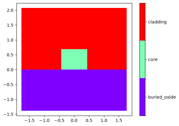
First, construct the geometry of waveguide according to figure 2d of the paper.
width = 0.88  # um
height = 0.69  # um

wavelength_range = [500, 2500]
wavelegnth_step = 50

# Construct waveguide geometry
core = shapely.geometry.box(-width / 2, 0, +width / 2, height)
cladding = shapely.geometry.box(-width * 2, 0, width * 2, height * 3)
buried_oxide = shapely.geometry.box(-width * 2, -height * 2, width * 2, 0)
polygon = OrderedDict(
    core=core,
    cladding=cladding,
    buried_oxide=buried_oxide,
)

# Define material property and resolution of waveguide
resolutions = dict(
    core={"resolution": 0.02, "distance": 0.3},
    cladding={"resolution": 0.05, "distance": 0.3},
    buried_oxide={"resolution": 0.05, "distance": 0.3},
)

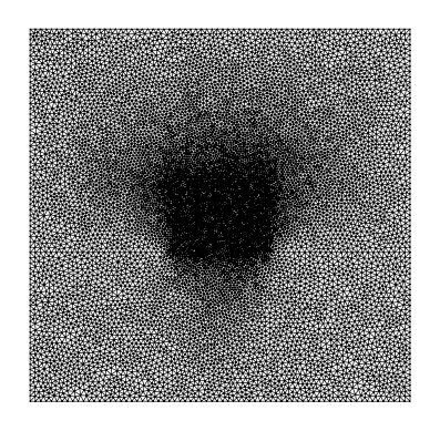
mesh = from_meshio(
    mesh_from_OrderedDict(polygon, resolutions, default_resolution_max=2)
)
mesh.draw().show()
plot_domains(mesh)
plt.show()
Use sellmeier equation to determine the refractive index of material.
def n_Si3N4(wavelength, fit=False):
    if wavelength >= 0.31 and wavelength <= 5.507:
        return math.sqrt(
            (3.0249 * wavelength**2) / (wavelength**2 - 0.1353406**2)
            + (40314 * wavelength**2) / (wavelength**2 - 1239.842**2)
            + 1
        )
    else:
        raise ValueError(
            f"wavelength provided is {wavelength}um, is out of the range for Si3N4"
        )


def n_SiO2(wavelength):
    if wavelength < 0.21 or wavelength > 6.7:
        raise ValueError(
            f"wavelength provided is {wavelength}um, is out of the range for {type}"
        )
    return np.sqrt(
        0.6961663 * wavelength**2 / (wavelength**2 - 0.0684043**2)
        + (0.4079426 * wavelength**2 / (wavelength**2 - 0.1162414**2))
        + (0.8974794 * wavelength**2 / (wavelength**2 - 9.896161**2))
        + 1
    )


n_dict = {"core": n_Si3N4, "cladding": n_SiO2, "buried_oxide": n_SiO2}
Create the mesh, and sweep wavelength using the same mesh. The target mode is te mode, so the mode is selected by highest te fraction
neff_list = []
aeff_list = []
basis0 = Basis(mesh, ElementTriP0())
epsilon = basis0.zeros()
wavelength_list = np.linspace(wavelength_range[0], wavelength_range[1], wavelegnth_step)

for wavelength in tqdm(wavelength_list):
    wavelength = wavelength * 1e-3
    for subdomain, n in n_dict.items():
        epsilon[basis0.get_dofs(elements=subdomain)] = n(wavelength) ** 2

    modes = compute_modes(basis0, epsilon, wavelength=wavelength, num_modes=3, order=1)
    modes_sorted = modes.sorted(key=lambda mode: -np.real(mode.te_fraction))
    mode = modes_sorted[0]

    neff_list.append(np.real(mode.n_eff))
    aeff_list.append(np.real(mode.calculate_effective_area()))
0%| | 0/50 [00:00<?, ?it/s]
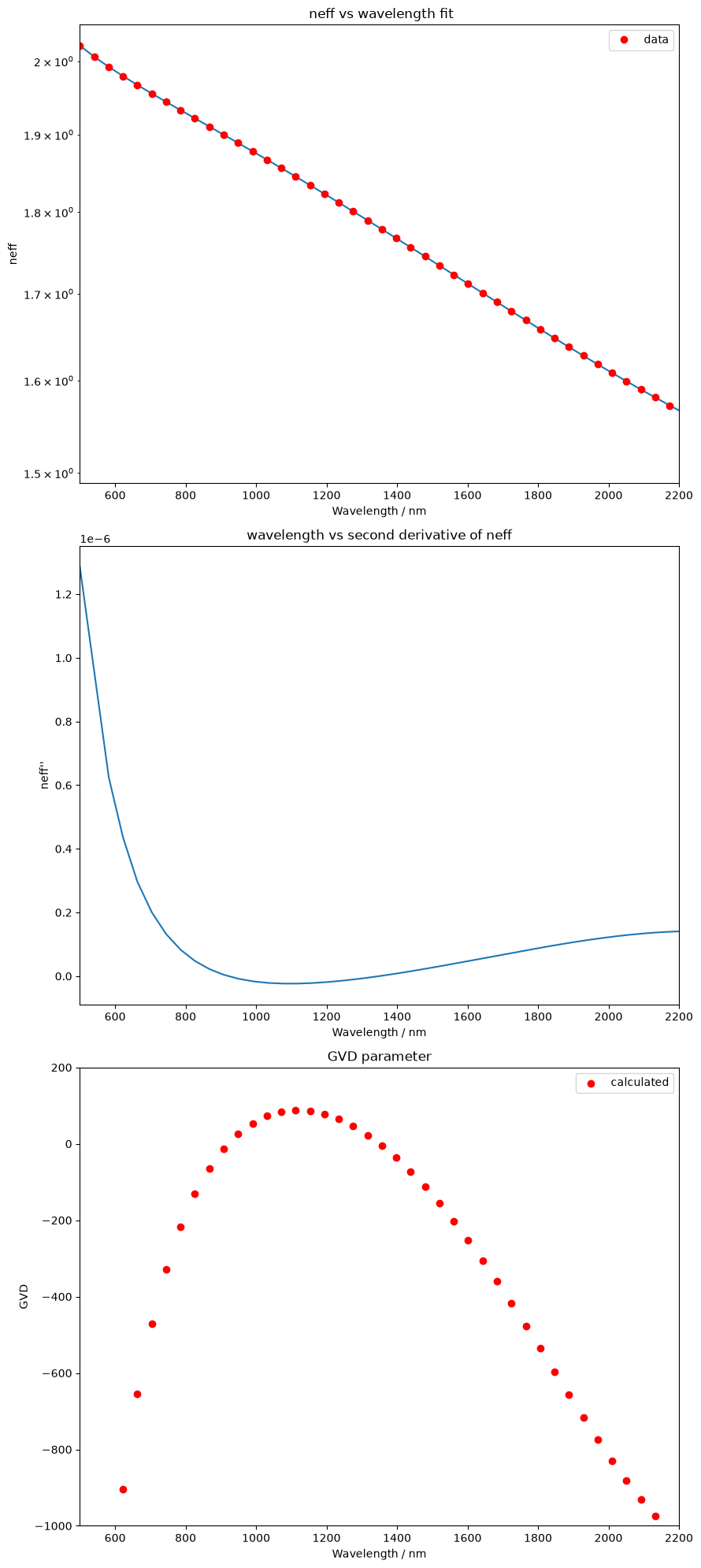
Calculate the GVD by fitting a curve for wavelength vs neff. Then take second derivative of the curve
y_spl = UnivariateSpline(wavelength_list, neff_list, s=0, k=3)
x_range = np.linspace(wavelength_list[0], wavelength_list[-1], 1000)
y_spl_2d = y_spl.derivative(n=2)

# Plot the result
fig, axs = plt.subplots(3, 1, figsize=(9, 20))

axs[0].set_xlabel("Wavelength / nm")
axs[0].set_ylabel("neff")
axs[0].set_title(" neff vs wavelength fit")
axs[0].semilogy(x_range, y_spl(x_range))
axs[0].semilogy(wavelength_list, neff_list, "ro", label="data")
axs[0].legend()
axs[0].set_xlim(500, 2200)

axs[1].set_xlabel("Wavelength / nm")
axs[1].set_ylabel("neff''")
axs[1].set_title("wavelength vs second derivative of neff")
axs[1].plot(x_range, y_spl_2d(x_range))
axs[1].set_xlim(500, 2200)

# ----Calculate and plot GVD
GVD = -wavelength_list / (2.99792e-7) * y_spl_2d(wavelength_list)
axs[2].scatter(wavelength_list, GVD, label="calculated", c="red")

axs[2].set_ylabel("GVD")
axs[2].set_xlabel("Wavelength / nm")
axs[2].set_ylim(-1000, 200)
axs[2].set_xlim(500, 2200)
axs[2].set_title("GVD parameter")
axs[2].legend()

plt.tight_layout()
plt.show()
Bibliography
-
Alexander Klenner and Aline S. Mayer and Adrea R. Johnson and Kevin Luke and Michael R. E. Lamont and Yoshitomo Okawachi and Michal Lipson and Alexander L. Gaeta and Ursula Keller, Gigahertz frequency comb offset stabilization based on supercontinuum generation in silicon nitride waveguides, Optics Express, 24(10):11043, 2016. doi:10.1364/OE.24.011043 ↩