Mode Sources and Monitors
We first launch a mode profile solved only at the center frequency, then repeat the straight-waveguide run with seven Chebyshev-sampled profiles selected through ModeSpec.num_freqs. This progression makes the broadband-source improvement directly visible. Finally, we reuse the broadband source for a simple width-step junction.
The simulation uses BeamZ's Design and Material API with its structure-aware rectilinear auto grid, including the native nonuniform mode solve, launch, monitor colocation, and area-weighted modal projection paths.
BeamZ is in beta
BeamZ is under active development. APIs, numerical behavior, and results may change between releases. Validate simulations independently before relying on them for design or production decisions.
Documentation note: The figures and text outputs embedded below are reference outputs bundled from the BeamZ v0.5.0 example notebooks (Apache-2.0). The code targets BeamZ v0.5.0; run the notebook to regenerate results for your local environment.
Setup
Import BeamZ together with the numerical and plotting libraries. The finite-difference mode solver is included in BeamZ.
import os
import sys
from dataclasses import replace
from pathlib import Path

import matplotlib.pyplot as plt
import numpy as np

try:
    from IPython.display import display
except ImportError:
    display = print

import beamz as bz

test_mode = os.environ.get("BEAMZ_DOCS_TEST") == "1"
plt.rcParams.update({"figure.dpi": 120})
print(f"Python: {sys.executable}")
print(f"BeamZ: {bz.__version__} ({Path(bz.__file__).resolve()})")
BEAMZ version: 0.4.2
Geometry, Band, and Grid
The design is a silicon strip waveguide on a silica substrate with air above it. Coordinates are centered on the simulation domain, so the source and monitor planes can be placed with simple signed offsets along x.
As in the reference, the monitors record 17 frequencies uniformly spaced from freq0 - 2*fwidth to freq0 + 2*fwidth. Setting ModeSpec.num_freqs=7 makes the broadband source use seven Chebyshev profile frequencies inside freq0 +/- 1.5*fwidth. plane_size = (0, 3 um, 2 um) means the source and mode-monitor planes are normal to x; the zero-sized dimension defines the propagation axis. GridSpec.auto refines the silicon interfaces and smoothly grades toward coarser cells away from the waveguide. The mode eigensolver receives the exact transverse edge arrays, and monitor overlaps use the corresponding physical cell-area weights.
# Define the unit length as micrometer
um = bz.um

# Height and width of the waveguide
wg_height = 0.22 * um
wg_width = 0.45 * um

# Permittivity of waveguide and substrate
si_eps = 3.48**2
sio2_eps = 1.45**2

# Free-space wavelength and frequency (in Hz)
lambda0 = 1.55 * um
freq0 = bz.LIGHT_SPEED / lambda0
fwidth = freq0 / 10

# Monitor 17 frequencies across +/- 2 fwidth.
# The broadband source itself uses 7 Chebyshev profiles across +/- 1.5 fwidth.
nfreqs = 3 if test_mode else 17
freqs = np.linspace(freq0 - 2 * fwidth, freq0 + 2 * fwidth, nfreqs)
lambdas_um = bz.LIGHT_SPEED / freqs / um
fcent_ind = nfreqs // 2

# Simulation size and PML thickness
sim_size = (
    (4.0 * um, 3.0 * um, 2.5 * um) if test_mode else (8.0 * um, 7.0 * um, 6.0 * um)
)
pml_t = (0.45 if test_mode else 1.25) * um
src_x = -sim_size[0] / 2 + pml_t + 0.75 * um
out_x = -src_x
plane_size = (0.0, 1.5 * um, 1.2 * um) if test_mode else (0.0, 3.0 * um, 2.0 * um)
run_time = 6 / freq0 if test_mode else 20 / fwidth
boundaries = (bz.PML(thickness=pml_t, formulation="cpml"),)

# Mode source and monitor specification
source_time = bz.GaussianPulse(
    freq0=freq0,
    fwidth=fwidth,
    offset=0.5 if test_mode else 4.0,
)
# Leave polarization unset so candidates retain descending-neff ordering.
# The fundamental source mode remains TE-like; setting polarization="te" here
# would reorder TE-like radiation candidates ahead of the former modes 1 and 2.
mode_spec = bz.ModeSpec(
    num_modes=1 if test_mode else 3, target_neff=0.98 * np.sqrt(si_eps)
)
broadband_profile_count = 3 if test_mode else 7

mode_grid_steps = 4 if test_mode else 10
grid_spec = bz.GridSpec.auto(
    wavelength=lambda0,
    min_steps_per_wvl=mode_grid_steps,
    max_scale=1.25,
)
Structures and Monitors
The straight reference simulation contains the substrate, the waveguide, and three monitors:
Monitorrecords the source-normalized frequency-domain field snapshotEy(x, y)at the central frequency.FluxMonitorcomputes the area-integrated Poynting flux through the output plane.ModeMonitordecomposes the same output-plane fields into forward and backward waveguide modes.
For a harmonic field, the signed power crossing a plane is
BeamZ reports this in watts after source-spectrum normalization, matching the convention used by the modal amplitudes.
# Materials
mat_air = bz.Material(permittivity=1.0)
mat_wg = bz.Material(permittivity=si_eps)
mat_sub = bz.Material(permittivity=sio2_eps)

# Initialize air background
design = bz.Design(background=mat_air)

# Add the silica substrate
design += bz.Box(
    center=(0, 0, -0.5 * sim_size[2]),
    size=(bz.inf, bz.inf, sim_size[2]),
    material=mat_sub,
)

# Add the silicon waveguide
design += bz.Box(
    center=(0, 0, 0.5 * wg_height),
    size=(bz.inf, wg_width, wg_height),
    material=mat_wg,
)

# Source plane
src_plane = bz.Box(center=(src_x, 0, 0.0), size=plane_size)
field_mnt = bz.FieldMonitor(
    center=(0.0, 0.0, 0.5 * wg_height),
    size=(sim_size[0], sim_size[1], 0.0),
    freqs=[freq0],
    fields=("Ey",),
    name="field",
)
flux_mnt = bz.FluxMonitor(
    center=(out_x, 0, 0.0), size=plane_size, freqs=freqs, name="flux"
)
mode_mnt = bz.ModeMonitor(
    center=(out_x, 0, 0.0),
    size=plane_size,
    freqs=freqs,
    mode_spec=mode_spec,
    name="mode",
)
Build and Inspect the Straight Simulation
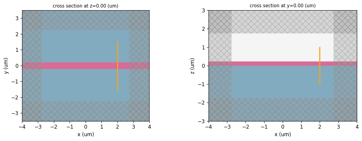
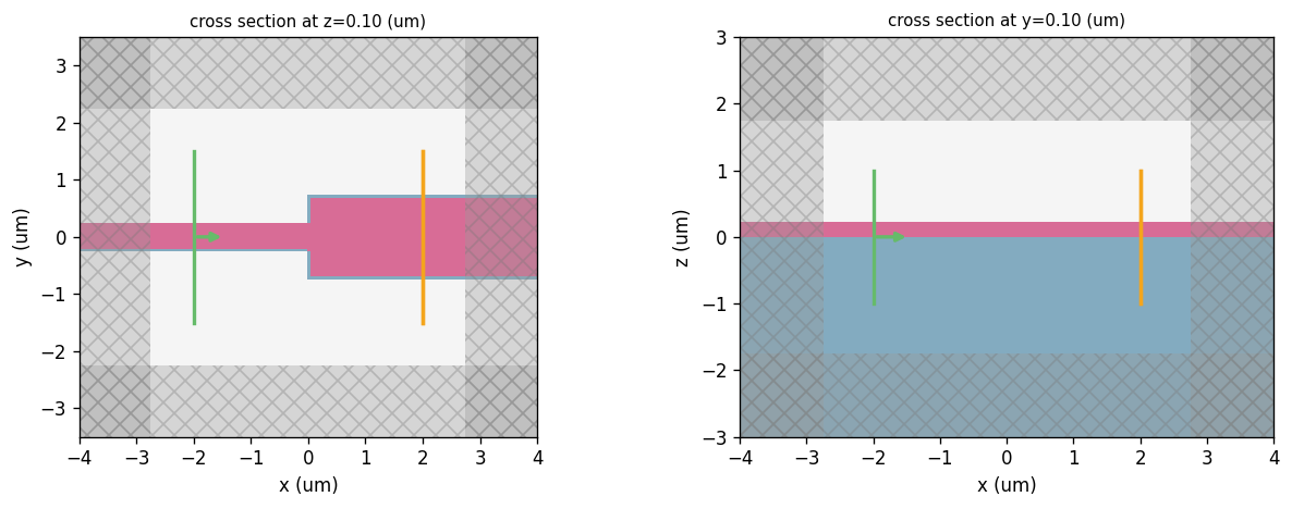
This first simulation has no source. It provides the geometry, realized rectilinear grid, and monitor planes used by the native ModeSource preview. The diagnostics below make the nonuniform mesh explicit by reporting each axis's cell count and spacing range. Plotting the cross sections is a quick check that the substrate, waveguide, source plane, and output monitor are where we expect them to be before running FDTD.
sim0 = bz.Simulation(
    domain=sim_size,
    grid_spec=grid_spec,
    design=design,
    sources=[],
    monitors=[field_mnt, flux_mnt, mode_mnt],
    boundaries=boundaries,
    run_time=run_time,
)
assert sim0.grid.metric_kind == "rectilinear"
print(
    f"grid = {sim0.grid.metric_kind}, shape = {sim0.grid.shape}, steps = {sim0.num_steps}"
)
for axis in ("x", "y", "z"):
    spacing = sim0.grid.cell_widths(axis) / um
    print(
        f"  {axis}: {spacing.size} cells, dl = {spacing.min():.3f}..{spacing.max():.3f} um"
    )
fig, axes = sim0.plot(z=0.0, y=0.0, show=False)
plt.show()
● Info: Auto-selecting 3D meshing for 3D design
● Rasterizing 3D structures...
● Rasterizing 3D structures... done (3/3)
● Info: 3D raster timing: setup=0.06s, structures=0.03s, pml=0.00s, total=0.14s
● Info: 3D raster kernels: fast_enabled=True, fast_rect=2, fast_poly=0, fallback=0
● Done: Created 3D mesh: 179 × 157 × 134 cells
● Info: Raster cache saved: fdabd4e253ff1b1c157a26403e712151df32e5f78286f97463b0e3b866da20d6.npz | save=0.47s
● Info: Rasterize wall-time: 0.14s | total=0.61s
dx = 0.045 um, steps = 12178
Solve Modes and Create the Center-Frequency Source
The native finite-difference mode solve finds fields of the form
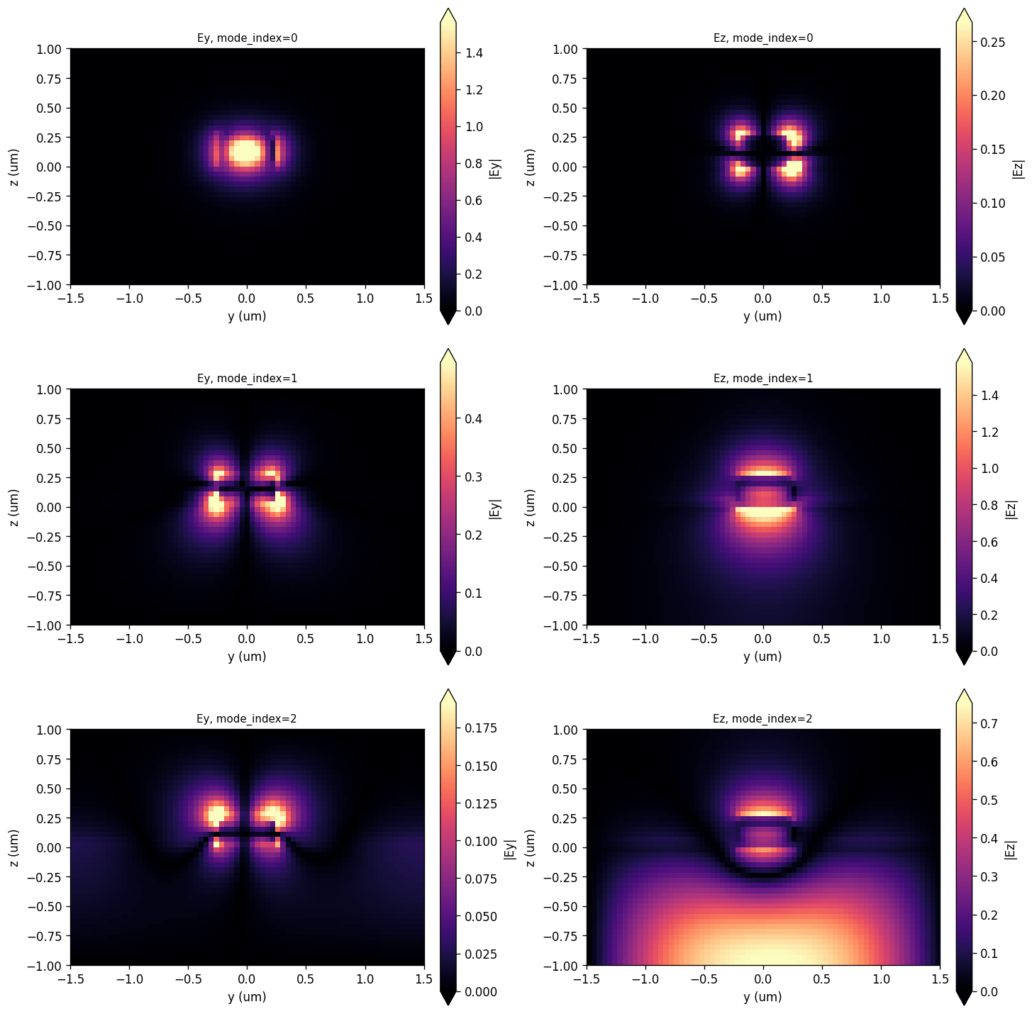
The table and field plots show all three requested eigensolver candidates. The plots use the stored transverse cell edges, so every colored rectangle occupies its true physical \(y\)-\(z\) area and the nonuniform spacing remains visible. Candidates below the substrate light line are radiation/finite-window modes rather than bound higher-order waveguide modes; the diagnostic below identifies them while retaining their profiles for inspection.
We convert the selected mode into a directional equivalent-current source. The selected mode is power-normalized so that, at the center frequency, the target launch power is
Here we inject the fundamental TE-like mode in the +x direction. The first source uses one profile at freq0, matching the first straight-waveguide run in the reference notebook.
mode_source_request = bz.ModeSource(
    center=src_plane.center,
    size=src_plane.size,
    direction="+",
    source_time=source_time,
    mode_spec=mode_spec,
)
modes = mode_source_request.solve_modes(sim0, freqs=[freq0])
assert np.all(np.isfinite(np.asarray(modes.neffs)))
from beamz.analysis import mode_data_to_dataframe
from beamz.analysis.plotting import plot_mode_field_components

mode_table = mode_data_to_dataframe(modes)
display(mode_table)

# A bound mode must lie above the highest surrounding-material light line.
cladding_neff = max(np.sqrt(mat_air.permittivity), np.sqrt(mat_sub.permittivity))
candidate_neffs = np.real(np.asarray(modes.neffs)[0])
candidate_mode_indices = tuple(range(candidate_neffs.size))
guided_mode_indices = tuple(
    int(index) for index in np.flatnonzero(candidate_neffs > cladding_neff + 1e-6)
)
if not guided_mode_indices:
    raise RuntimeError("No guided mode was found above the cladding light line.")
radiation_mode_indices = tuple(
    int(index) for index in np.flatnonzero(candidate_neffs <= cladding_neff + 1e-6)
)
if radiation_mode_indices:
    print(
        f"Candidate modes {radiation_mode_indices} are plotted for inspection, but "
        f"indices are at or below the cladding light line ({cladding_neff:.4g})."
    )

fig, axes, neffs = plot_mode_field_components(
    modes,
    field_names=("Ey", "Ez"),
    mode_indices=candidate_mode_indices,
    val="abs",
    f=freq0,
    figsize=(12, 4 * len(candidate_mode_indices)),
    show=False,
)
plt.show()

# The first run uses exactly one mode profile at freq0. The separate
# seven-frequency broadband reconstruction is constructed below.
mode_source_single = mode_source_request.updated_copy(
    mode_spec=replace(mode_source_request.mode_spec, num_freqs=1),
)
single_profile_freqs = mode_source_single.profile_frequencies()
np.testing.assert_allclose(single_profile_freqs, [freq0])
print("Single-profile frequency (THz):", single_profile_freqs[0] * 1e-12)
sim_single = sim0.updated_copy(sources=(mode_source_single,))
Center-Frequency Source: Straight Waveguide
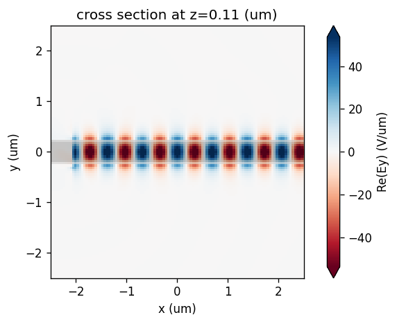
We first run the source whose spatial profile was solved only at freq0. The in-plane field plot is a frequency-domain DFT snapshot at freq0; BeamZ source-normalizes this plot and displays electric fields in V/um.
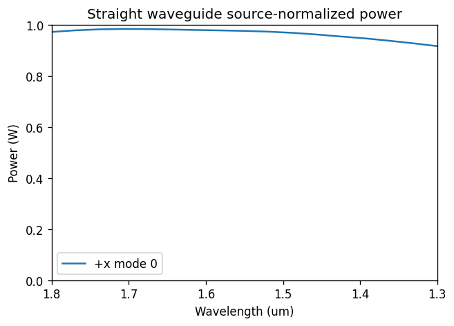
The straight waveguide acts as a reference run: ideally nearly all power should remain in the forward fundamental mode, with very little backward power.
sim_data_single = sim_single.run(progress=not test_mode)
sim_data_single.plot_field(
    "field",
    "Ey",
    frequency=freq0,
    val="real",
    cmap="RdBu",
    xlim=(-2.5, 2.5),
    ylim=(-2.5, 2.5),
    show_grid=True,
)
plt.show()
● JIT compiling v0.3 packed FDTD program... done!
● Progress: 100% (12178/12178 steps)
Center-Frequency Source: Power and Mode Decomposition
The mode monitor expands the recorded fields in a power-normalized modal basis. BeamZ returns source-normalized frequency-domain responses by default, so the source pulse envelope is divided out. For the one-profile source, a single straight-waveguide scale makes the largest measured power exactly 1 W; this preserves its physical frequency dependence without allowing the small off-center numerical overshoot to exceed the requested power.
The raw acquisition remains available through SimulationResults.renormalize(None). We plot that pulse-weighted spectrum beside the source-normalized response, applying the same one-watt center-frequency convention to make their different shapes directly comparable. This works for analytic and sampled source waveforms without reconstructing a Gaussian by hand.
def scalar_power_scale(values, target_power, *, reference_index=None):
    """Return one scale using either a selected bin or the spectral peak."""
    spectrum = np.asarray(values, dtype=float)
    reference = float(
        np.max(spectrum) if reference_index is None else spectrum[reference_index]
    )
    if not np.isfinite(reference) or reference <= 0.0:
        raise RuntimeError("Straight-waveguide reference power must be positive.")
    return float(target_power) / reference


def spectral_power_scale(values, target_power):
    """Return a per-frequency straight-waveguide reference scale."""
    spectrum = np.asarray(values, dtype=float)
    if np.any(~np.isfinite(spectrum)) or np.any(spectrum <= 0.0):
        raise RuntimeError("Straight-waveguide reference spectrum must be positive.")
    return float(target_power) / spectrum


flux_single_response = np.asarray(sim_data_single["flux"].flux, dtype=float)
mode_amps_single = sim_data_single.mode("mode")
coeffs_f_single = mode_amps_single.amps.sel(direction="+")
coeffs_b_single = mode_amps_single.amps.sel(direction="-")
single_power_scale = scalar_power_scale(flux_single_response, mode_source_single.power)
flux_single = flux_single_response * single_power_scale
mode_power_f_single = np.abs(coeffs_f_single.values) ** 2 * single_power_scale
mode_power_b_single = np.abs(coeffs_b_single.values) ** 2 * single_power_scale

raw_single = sim_data_single.renormalize(None)
flux_single_raw = np.asarray(raw_single["flux"].flux, dtype=float)
mode_amps_single_raw = raw_single.mode("mode")
pulse_power_scale = scalar_power_scale(
    flux_single_raw, mode_source_single.power, reference_index=fcent_ind
)
flux_single_pulse = flux_single_raw * pulse_power_scale
mode_power_f_single_pulse = (
    np.abs(mode_amps_single_raw.amps.sel(direction="+").values) ** 2 * pulse_power_scale
)
assert np.all(np.isfinite(flux_single))
assert np.all(np.isfinite(flux_single_pulse))
assert np.all(np.isfinite(mode_power_f_single))
np.testing.assert_allclose(np.max(flux_single), mode_source_single.power, rtol=1e-12)
np.testing.assert_allclose(
    flux_single_pulse[fcent_ind], mode_source_single.power, rtol=1e-12
)

print("Peak source-normalized flux:", float(np.max(flux_single)))
print("Source-normalized flux at central frequency:", float(flux_single[fcent_ind]))
print("Pulse-weighted flux at central frequency:", float(flux_single_pulse[fcent_ind]))
print("Power distribution at central frequency in first three modes")
print("  positive dir.", mode_power_f_single[fcent_ind])
print("  negative dir.", mode_power_b_single[fcent_ind])
fig, axes = plt.subplots(1, 2, figsize=(11, 4), sharey=True)
for ax, title, total_power, mode0_power in (
    (axes[0], "Source-normalized response", flux_single, mode_power_f_single[:, 0]),
    (
        axes[1],
        "Pulse-weighted spectrum",
        flux_single_pulse,
        mode_power_f_single_pulse[:, 0],
    ),
):
    ax.plot(lambdas_um, total_power, label="Total flux")
    ax.plot(lambdas_um, mode0_power, label="+x mode 0")
    ax.axhline(1.0, color="black", linewidth=0.8, alpha=0.5)
    ax.axvspan(
        bz.LIGHT_SPEED / (freq0 + 1.5 * fwidth) / um,
        bz.LIGHT_SPEED / (freq0 - 1.5 * fwidth) / um,
        color="black",
        alpha=0.08,
        label="future broadband design band",
    )
    ax.set_xlim([lambdas_um[-1], lambdas_um[0]])
    ax.set_xlabel("Wavelength (um)")
    ax.set_title(title)
    ax.legend(fontsize=8)
axes[0].set_ylabel("Power (W), referenced to 1 W at 1.55 um")
fig.suptitle("Single-profile mode source")
fig.tight_layout()
plt.show()
Broadband Mode Source: Chebyshev Profiles
The broadband source uses seven frequency-dependent profiles. We set num_freqs on the source's immutable ModeSpec; BeamZ derives the Chebyshev profile frequencies from the pulse center and width and reconstructs the frequency-dependent equivalent-current profile during compilation.
The plot below makes that interpolation explicit. The weights sum to one at every frequency, are cardinal at the seven solve frequencies, and can be negative between nodes—as expected for polynomial rather than piecewise-linear interpolation. Frequencies outside the sampled interval use the nearest end profile because broadband accuracy is only promised inside the shaded design band.
# Configure broadband reconstruction through ModeSpec, then inspect the
# exact public profile frequencies that ModeSource will compile.
mode_source_bb = mode_source_request.updated_copy(
    mode_spec=replace(mode_source_request.mode_spec, num_freqs=broadband_profile_count),
)
profile_freqs = mode_source_bb.profile_frequencies()
profile_lambdas_um = bz.LIGHT_SPEED / profile_freqs / um


def barycentric_partition_weights(sample_freqs, nodes):
    """Return the polynomial partition associated with frequency nodes."""
    nodes = np.asarray(nodes, dtype=float)
    samples = np.clip(np.asarray(sample_freqs, dtype=float), nodes[0], nodes[-1])
    differences = nodes[:, None] - nodes[None, :]
    np.fill_diagonal(differences, 1.0)
    barycentric = 1.0 / np.prod(differences, axis=1)
    weights = np.empty((nodes.size, samples.size), dtype=float)
    for sample_index, sample in enumerate(samples):
        delta = sample - nodes
        exact = np.flatnonzero(
            np.isclose(delta, 0.0, rtol=0.0, atol=8 * np.finfo(float).eps * nodes[-1])
        )
        if exact.size:
            weights[:, sample_index] = 0.0
            weights[exact[0], sample_index] = 1.0
        else:
            values = barycentric / delta
            weights[:, sample_index] = values / values.sum()
    return weights


interp_weights = barycentric_partition_weights(freqs, profile_freqs)
cardinal_weights = barycentric_partition_weights(profile_freqs, profile_freqs)

np.testing.assert_allclose(interp_weights.sum(axis=0), 1.0, atol=1e-12)
np.testing.assert_allclose(
    cardinal_weights, np.eye(broadband_profile_count), atol=1e-12
)
print("Chebyshev profile wavelengths (um):")
print(np.round(profile_lambdas_um, 6))
print(
    "maximum partition-of-unity error:",
    np.max(np.abs(interp_weights.sum(axis=0) - 1.0)),
)

fig, ax = plt.subplots(figsize=(6, 4))
for index, weight in enumerate(interp_weights):
    ax.plot(lambdas_um, weight, marker=".", label=f"profile {index}")
ax.axhline(0.0, color="black", linewidth=0.6)
ax.set_xlim([lambdas_um[-1], lambdas_um[0]])
ax.set_xlabel("Wavelength (um)")
ax.set_ylabel("Polynomial interpolation weight")
ax.set_title("Seven-profile Chebyshev reconstruction")
ax.legend(ncol=2, fontsize=8)
plt.show()
Broadband Mode Source: Straight Waveguide
We now rerun the unchanged straight waveguide with the seven-profile source. The source compiler power-normalizes every solved profile using the mode solver's exact transverse metric. We then apply the straight-waveguide flux as a per-frequency reference, so the broadband total power is exactly 1 W while the mode curves continue to expose launch purity and residual modal content. This reference normalization is independent of the temporal pulse envelope.
sim_bb = sim0.updated_copy(sources=(mode_source_bb,))
sim_data_bb = sim_bb.run(progress=not test_mode)

flux_bb_response = np.asarray(sim_data_bb["flux"].flux, dtype=float)
mode_amps_bb = sim_data_bb.mode("mode")
coeffs_f_bb = mode_amps_bb.amps.sel(direction="+")
coeffs_b_bb = mode_amps_bb.amps.sel(direction="-")
bb_power_scale = spectral_power_scale(flux_bb_response, mode_source_bb.power)
flux_bb = flux_bb_response * bb_power_scale
mode_power_f_bb = np.abs(coeffs_f_bb.values) ** 2 * bb_power_scale[:, None]
mode_power_b_bb = np.abs(coeffs_b_bb.values) ** 2 * bb_power_scale[:, None]
assert np.all(np.isfinite(flux_bb))
assert np.all(np.isfinite(mode_power_f_bb))
np.testing.assert_allclose(flux_bb, mode_source_bb.power, rtol=1e-12)
design_band = np.abs(freqs - freq0) <= 1.5 * fwidth

print("Broadband flux at central frequency:", float(flux_bb[fcent_ind]))
print("Broadband power distribution at central frequency")
print("  positive dir.", mode_power_f_bb[fcent_ind])
print("  negative dir.", mode_power_b_bb[fcent_ind])
print(
    "Broadband mode-0 range in design band:",
    mode_power_f_bb[design_band, 0].min(),
    mode_power_f_bb[design_band, 0].max(),
)

fig, ax = plt.subplots(figsize=(6, 4))
ax.plot(lambdas_um, flux_single, label="Total (single profile)")
ax.plot(lambdas_um, flux_bb, label="Total (broadband)")
ax.plot(lambdas_um, mode_power_f_single[:, 0], "x--", label="Mode 0 (single profile)")
ax.plot(lambdas_um, mode_power_f_bb[:, 0], ".--", label="Mode 0 (broadband)")
ax.axhline(1.0, color="black", linewidth=0.8, alpha=0.5)
ax.axvspan(
    bz.LIGHT_SPEED / (freq0 + 1.5 * fwidth) / um,
    bz.LIGHT_SPEED / (freq0 - 1.5 * fwidth) / um,
    color="black",
    alpha=0.08,
    label="+/- 1.5 fwidth",
)
ax.set_xlim([lambdas_um[-1], lambdas_um[0]])
ax.set_xlabel("Wavelength (um)")
ax.set_ylabel("Power (W)")
ax.set_title("Single-profile and broadband mode sources")
ax.legend(fontsize=8)
plt.show()
Signed Flux and Modal-Power Accounting
The curves labeled Total above are signed Poynting flux, not a sum of the positive-direction modal powers. Forward modal power contributes positively and backward modal power negatively. Therefore a forward mode-0 curve can lie above the signed-flux curve without implying that the flux calculation is wrong.
For a complete lossless modal basis, flux = sum(P_forward) - sum(P_backward). Here we request only three modes, so flux - net_guided also contains radiation, modes outside the requested basis, finite-aperture projection residual, and discretization error. The source has only one scalar amplitude: rescaling it cannot independently force both the fundamental-mode power and the total signed flux to exactly 1 W when that residual is nonzero.
This cell applies the same straight-waveguide reference scales to the independently recorded, source-normalized FluxMonitor and ModeMonitor, prints the accounting, and plots signed flux against net power in modes 0–2. It can be run after the simulations above without rerunning FDTD.
def power_accounting(
    label, flux, mode_data, power_forward, power_backward, power_scale
):
    flux_values = np.asarray(flux, dtype=float)
    mode_monitor_flux = np.asarray(mode_data.flux.values, dtype=float) * power_scale
    net_guided = power_forward.sum(axis=1) - power_backward.sum(axis=1)
    unresolved = flux_values - net_guided
    center = fcent_ind

    print(label)
    print(f"  signed flux:              {flux_values[center]:.9f} W")
    print(f"  forward mode 0:           {power_forward[center, 0]:.9f} W")
    print(f"  net power in modes 0-2:  {net_guided[center]:.9f} W")
    print(f"  unresolved signed flux:  {unresolved[center]:.9f} W")
    print(
        f"  max flux-monitor difference: {np.max(np.abs(flux_values - mode_monitor_flux)):.3e} W"
    )
    return net_guided, unresolved


net_guided_single, unresolved_single = power_accounting(
    "Single-profile source",
    flux_single,
    mode_amps_single,
    mode_power_f_single,
    mode_power_b_single,
    single_power_scale,
)
net_guided_bb, unresolved_bb = power_accounting(
    "Broadband source",
    flux_bb,
    mode_amps_bb,
    mode_power_f_bb,
    mode_power_b_bb,
    bb_power_scale,
)

fig, axes = plt.subplots(1, 2, figsize=(11, 4), sharey=True)
for ax, title, flux, mode0, net_guided in (
    (
        axes[0],
        "Single profile",
        flux_single,
        mode_power_f_single[:, 0],
        net_guided_single,
    ),
    (axes[1], "Broadband", flux_bb, mode_power_f_bb[:, 0], net_guided_bb),
):
    ax.plot(lambdas_um, flux, label="Signed Poynting flux")
    ax.plot(lambdas_um, mode0, label="Forward mode 0")
    ax.plot(lambdas_um, net_guided, "--", label="Net modes 0-2")
    ax.axhline(1.0, color="black", linewidth=0.7, alpha=0.5)
    ax.set_xlim([lambdas_um[-1], lambdas_um[0]])
    ax.set_xlabel("Wavelength (um)")
    ax.set_title(title)
axes[0].set_ylabel("Power (W)")
axes[0].legend(fontsize=8)
plt.show()
Width-Step Junction
The junction variant keeps the broadband source and monitor definitions, but replaces the output half of the waveguide with a wider guide. This creates a simple discontinuity where the input mode can scatter into radiation and into several modes of the wider section. Using the matching broadband straight run as the reference avoids adding a fourth full simulation.
wgout_width = 1.4 * um
design_jct = design.with_structure(
    bz.Box(
        center=(0.25 * sim_size[0], 0, 0.5 * wg_height),
        size=(0.5 * sim_size[0], wgout_width, wg_height),
        material=mat_wg,
    )
)

sim_jct0 = bz.Simulation(
    domain=sim_size,
    grid_spec=grid_spec,
    design=design_jct,
    sources=[],
    monitors=[field_mnt, flux_mnt, mode_mnt],
    boundaries=boundaries,
    run_time=run_time,
)
sim_jct_bb = sim_jct0.updated_copy(sources=(mode_source_bb,))
fig, axes = sim_jct_bb.plot(z=0.1 * um, y=0.1 * um, width_ratios=[1, 1.4], show=False)
plt.show()
● Info: Auto-selecting 3D meshing for 3D design
● Rasterizing 3D structures...
● Rasterizing 3D structures... done (4/4)
● Info: 3D raster timing: setup=0.03s, structures=0.02s, pml=0.00s, total=0.06s
● Info: 3D raster kernels: fast_enabled=True, fast_rect=3, fast_poly=0, fallback=0
● Done: Created 3D mesh: 179 × 157 × 134 cells
● Info: Raster cache saved: 3a6d5f41dcb765a7bc75c47eed1da9f824dd0aea6f5d26bd8c61fb898a0d2171.npz | save=0.51s
● Info: Rasterize wall-time: 0.06s | total=0.57s
sim_data_jct_bb = sim_jct_bb.run(progress=not test_mode)
print(f"completed {sim_jct_bb.num_steps} FDTD steps")
● JIT compiling v0.3 packed FDTD program... done!
● Progress: 100% (12178/12178 steps)
completed 12178 FDTD steps
Junction Fields and Normalized Mode Powers
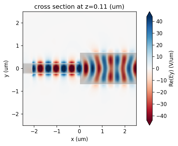
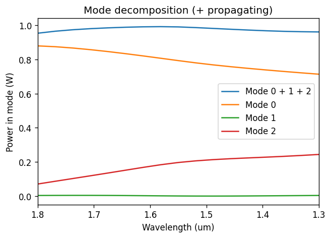
The field snapshot shows the interference and spreading after the width step. For the modal plot, the junction amplitudes are normalized by the matching broadband straight-waveguide flux, exactly as a reference-run normalization removes residual launch and discretization error.
If the computed modal powers do not sum to one, the missing part is power scattered into radiation, reflected modes, modes outside the requested basis, or numerical loss.
sim_data_jct_bb.plot_field(
    "field",
    "Ey",
    frequency=freq0,
    val="real",
    cmap="RdBu",
    xlim=(-2.5, 2.5),
    ylim=(-2.5, 2.5),
    show_grid=True,
)
plt.show()

amps_jct_bb = sim_data_jct_bb.mode("mode").amps.sel(direction="+")
amps_jct_bb = amps_jct_bb / np.sqrt(np.maximum(flux_bb_response, 1e-18))[:, None]

fig, ax = plt.subplots(1, figsize=(6, 4))
ax.plot(lambdas_um, np.sum(np.abs(amps_jct_bb.values) ** 2, axis=1))
ax.plot(lambdas_um, np.abs(amps_jct_bb.values) ** 2)
ax.set_xlim([lambdas_um[-1], lambdas_um[0]])
ax.set_xlabel("Wavelength (um)")
ax.set_ylabel("Power in mode (W)")
ax.set_title("Mode decomposition (+ propagating)")
ax.legend(["Mode 0 + 1 + 2", "Mode 0", "Mode 1", "Mode 2"])
plt.show()