Introduction
The vbias tool is used to shrink GDS shapes according to their thickness. It is
predominantly intended to be used as a CLI tool, but some public functions are
available.
Quick Index
Quick Start
To run vbias on a gds file with default settings, you can just run:
vbias input.gds
This will create a new GDS file called biased.gds.
However, you can also specify options to the vbias cli:
vbias input.gds -o output.gds -l 6/0 -I 10/0 -E 10/1 -c 0.05,-0.04
This will run the biasing on input.gds and save the biased version to output.gds.
Polygons on layer 6/0 will be considered for biasing if they are under the
inclusion layer 10/0 but not under the exclusion layer 10/1. The width of each
polygon (distance between vertex and the closed point at the opposite side of the
polygon) will be reduced by the bias delta equation:
$$
\Delta=0.05 - 0.04 * x
$$
To understand some of the flags better and get some insight in the algorithm, please
have a look at the algorithm overview. You can also get more info on
all available cli flags here, or run vbias --help
The biasing algorithm considers each cell individually, hence inclusion and exclusion layers are only considered if they are at exactly the same hierarchy level as the polygons to bias! You can circumvent this limitation by flattening the GDS.
Algorithm
For an in-depth algorithm overview, click here!
The variable biasing algorithm can roughly be described by the following steps:
- Read the gds file into cells containing simple polygons boundaries.
- Select the relevant boundaries for updates (the layer to bias is determined
-lcli flag.) - Merge polygons into bigger polygons where possible and combine those merged polygons into a collection of polygons for which none of the polygons touch (as otherwise they would have been merged together).
- Apply variable bias on the exterior and each of the interiors of each of the polygons in the multi polygon: see Algorithm.
- Convert the biased polygons back into simple polygon boundaries with no holes, possibly adding fracture lines to do so.
- Save the GDS file
- Sync with KLayout viewer (if the viewer is open).
The core of the biasing of a single polygons can be summarized as follows:
- Convert the exterior and interior into line strings with counter-clockwise and clockwise winding respectively.
- Loop through each point in each line string
- For each point find the closest point on the closest edge segment on either the same line string or any other line string which still belongs to the same polygon, taking into account a bunch of filtering conditions.
- Use the distance between the point and the edge segment to calculate the bias delta.
- Move the point by the calculated bias delta amount in the direction of the opposite point.
what's described above is just a shortened version of the whole story. Read the full algorithm walkthrough here.
Algorithm Overview
Jump to section:
- Merging polygons
- Parallelization
- Polygon simplification
- Biasing algorithms
- Grid Fracturing
- Vertex bias direction
- Biasing algorithms
- Filtering Conditions
- Interpolation
- Bias Delta Equation
- Debug Mode
Merging polygons
We first convert all the GdsBoundary elements into polygons. Note that those polygons
might have unwanted fracture lines in them, as GDS files don't support polygons with
holes:
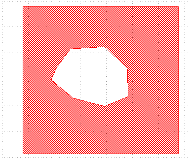
Fracture lines are not desirable as they are basically virtual edges, which, when biased, will introduce actual gaps in the geometry.
We therefore need to merge the GdsBoundary elements as they are in the GDS into
Polygons, possibly containing holes. Any touching polygons will be merged together into
a bigger polygon and all undesirable fracture lines will disappear.
Parallelization
Most GDS layers that will be biased will contain many polygons to bias. The algorithm is parallelized over the available polygons in the layer.
This works, as we already merged all touching polygons together, so any bias that needs to be applied to a certain point will guaranteed be coming from an 'opposite' point on the same polygon.
Polygon simplification
To avoid having to bias too many vertices, each polygon is simplified using the Ramer-Douglas-Peucker algorithm.
Grid fracturing
We fracture a copy of the polygon on a grid. This fractured polygon will be used to find the paired edge which determines the distance to be biased. Fracturing the grid in advance allows us to only consider edges in the vicinity of the current point as 'opposites'. Note that it is still the original polygon that is biased! We're only using the fractured polygon to reduce the search space to find opposite edges.
-g is the CLI flag to change the grid cell size. Note that this should be at least
the minimum width that is biased. The minimum bias width can be determined by the
(first) zero of the polynomial bias function (given by the -c flag).
In this step we're basically instantiating a grid which stores the centers of the grid cells and the edge crossing locations. We then use that information to fracture the polygon on a grid, as can be seen in the image below:
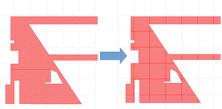
It will still be the original polygon that will be biased! We're only going to use the fractured polygon to reduce the search space to find opposite edges while iterating over each point to bias in the original polygon.
The goal will now be to iterate over each point in the original non-fractured polygon. By using the location of the point to bias we can select the grid-cell to which the current point belongs. Assuming that each grid cell is bigger than the minimum to-bias distance we'll know for sure that any opposite edge should be in the current grid cell or one of its neighbors.
Vertex bias direction
For each polygon we iterate over each vertex in its boundary (outer boundary and possible hole boundaries too). We're also keeping track of the neighboring vertices.
For each of those vertices, we will try to find the closest edge on the opposite side of the polygon. We'll recognize multiple cases that require a slightly different way of biasing, depending on which angle we're seeing around the current point.
Let's now have a look at the angle
$$\theta \in \left[ 0, 2\pi \right)$$
between the incoming edge and the outgoing edge at the current point to bias. We can split it up into 5 distinct angle regions:
-
θ < 90°: We're looking at a concave position in the polygon: the to-bias region is outside of a V-like shape. Such a point should probably not be biased as the bias direction would be too parallel with both the incoming and outgoing edge. Moreover, sharp angles should probably not be present in our GDS anyway.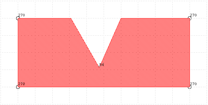 .
. -
θ ≈ 90°: We're looking at a concave right angle in the polygon. The problem with such a point is that it effectively belongs to two perpendicular edges. The approach used here is to calculate the bias delta for the incoming edge and the bias delta for the outgoing edge and select the largest resulting bias delta.-ris the CLI flag to change the 'right angle tolerance', i.e. the amount of deviation from 90° to consider an angle still to be a right angle.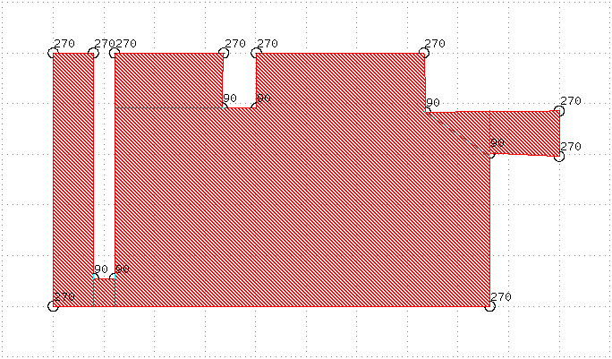
-
90°<θ<270°: This is the most common case: we're looking at a (quasi) straight edge, where (at least locally) the incoming angle is approximately equal to the outgoing angle. We'll look for another edge with a certain viewing cone leaving from the point to bias.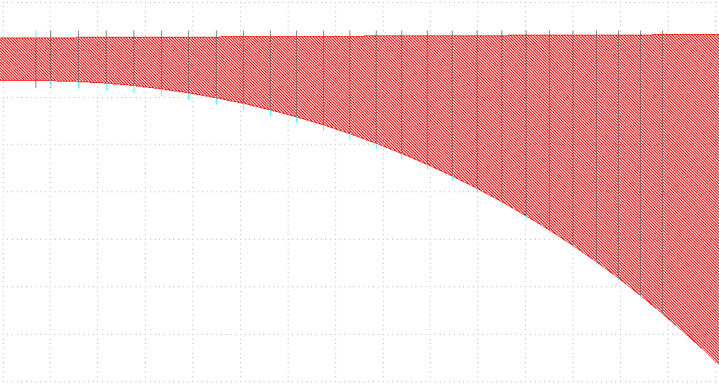
-
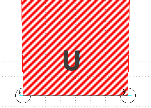
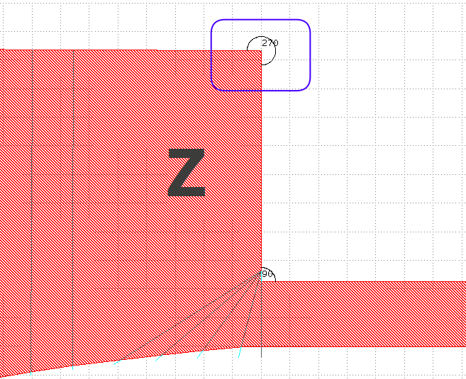
θ≈270°: This convex right angle case needs special care as it's a common termination in components like in MMIs. We can discern two cases: a U-like shape and a Z-like shape. We'll want to bias the U-like shape as it has two parallel edges, but Z-like shapes we'll need to leave alone:This is a U-like shape common in mmis: the two edges need to come closer together.
This is a Z-like shape: the (circled in blue) point should (probably) not be biased as the next edge does not fold back.
-
270°<θ<360°: This is again a sharp angle and should probably not be present in the GDS, hence we will not bias it .
Biasing algorithms
Since we're ignoring both concave and convex sharp-angle cases and since the θ≈90°
relies on having two edge-biasing steps, we can basically discern two independent
biasing algorithms:
- Edge bias: used for 99% of all points to bias
- Convex right angle bias: used in very specific cases (U-like terminations)
Let's go a bit deeper in both those algorithms...
1. Edge Bias
- For each point on the unfractured polygon, find the grid cell to which the point belongs in the fractured polygon together with all the neigboring cells.
- Get all edges from the polygons in the current grid cell and the 8 neighboring grid cells: those are the candidate 'receiver' edges.
- Iterate over all found edges.
- Find the closest point on the current edge being considered with respect to the current point being biased. Note that we considerably reduced the number of edges to check for by fracturing our polygon on a grid.
- Check the filtering conditions for the opposite point we found. If the opposite point passes all the filtering conditions it means that the opposite point we found is currently the best option to bias towards. We save the point.
- Once we went through all the possible opposite line segments. Use the distance between the vertex being biased and the best opposite point we found to calculate the bias delta.
- Move the point by the calculated bias delta amount in the direction of the opposite point.
2. Convex right angle Bias
When we're at a convex right angle we'll need to have a different approach as we might wwant to bias along the edge, which is impossible in the normal edge-bias algorithm as we limit ourselves to a certain viewing cone.
We therefore look at the next point on the line string, which by definition will be in the perpendicular direction compared to the edge made by the previous point and the current point. We look at what bias this point would give.
Then we do the opposite: we look at the previous point on the line string, which by definition will be in the perpendicular direction compared to the edge made by the next point and the current point. We look at what bias this point would give.
Then we select the point with the largest bias and bias in that direction.
Filtering Conditions
An 'opposite' point will be considered invalid when one of the following checks fails.
- The distance to the 'opposite' point is zero: the 'opposite' point is the same point as the point being biased, hence invalid.
- The distance to the opposite point is larger than the minimum distance we've found so far: the 'opposite' point is farther away and will result in less bias then what we've found so far, hence irrelevant.
- The 'opposite' point is a point on one of the virtual edges of the grid we just created: virtual edges are not real and should not be considered, hence invalid.
- The line from the current point to the opposite point is not in the viewing cone of the current point: invalid.
- The line from the opposite point to the current point is not in the viewing angle of the opposite point: invalid.
- The line from the current point to the opposite point crosses a polygon hole ore more generally leaves the current polygon being considered: invalid.
When one check fails we don't need to check any other checks. The above checks are hence more or less ordered from 'least expensive' to 'most expensive' computation-wise.
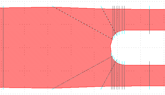
Interpolation
This is almost the complete story, but we forgot one thing: edge interpolation.
Sometimes we'll have very long straight edges which still need a different bias compared to where on the edge you are. Consider for example the following cellure:
With the currently described biasing algorithm only the currently present vertices will be biased:

However, the bottom edge should also be biased towards the removed half circle. To be able to do this we need to enable interpolation.
This looks more like it.
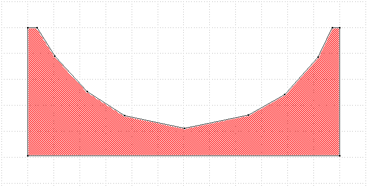
Bias Delta Equation
Each edge gets the following polynomial bias:
$$ \Delta = c_0 + c_1 x + c_2 x^2 + ... c_n x^n $$
The bias describes how the thickness of a polygon gets reduced, hence each biased vertex of a polygon gets moved in the direction of the opposite edge by half that amount.
The -c flag can be used to specify an arbitray number of polynomial coefficients for the
biasing. The coefficients should be given in ascending order of the polynomial (starting
at 0) and should be comma-separated.
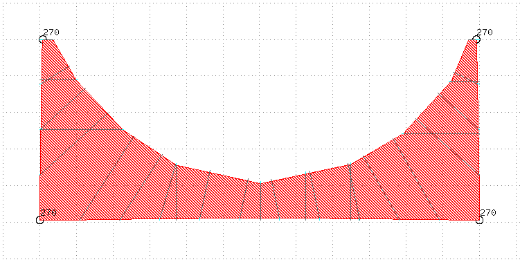
Debug Mode
When running vbias in debug mode, we will keep track of debug
elements. Debug elements are annotations which will be patched into the GDS Cell on
save. This gives an insight in how a vertex was classified and biased. Have a look at
the following y-splitter image:
What we're seeing here is black lines connecting the original point with its original 'opposite' pair edge. The cyan line heads signify how the original point was moved.
Further to the right of the gds, we can see angle annotations:
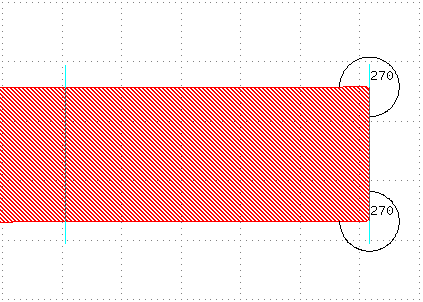
As we discussed here, sometimes the angle around a certain point determines how the point will be biased.
CLI
Variable bias CLI

Usage: vbias [OPTIONS] <PATH>

Arguments:
  <PATH>
          The path to the gds file to read

Options:
  -o, --output-path <OUTPUT_PATH>
          The path to the gds file to read

          [default: biased.gds]

  -O, --keep-orig
          Copy the original layer into the output GDS (easy for comparing old v new)

  -D, --debug
          Enable debug mode

          Activating debug mode will introduce a bunch of debug shapes into the biased gds. Moreover all unmodified layers will be dropped.

  -t, --threads <THREADS>
          Default number of threads used (set to 0 for max number of threads)

          [default: 0]

  -v, --viewing-angle <VIEWING_ANGLE>
          Default viewing angle (in degrees).

          The viewing angle is the maximum allowed angle with the normal at an edge point under which we're allowed to look for an edge close enough for biasing.

          [default: 80]

  -r, --right-angle-tolerance <RIGHT_ANGLE_TOLERANCE>
          Default right-angle tolerance (in degrees).

          The right angle tolerance signifies the deviation from 90° under which an angle is still considered a right-angle.

          [default: 25]

  -e, --rdp-eps <RDP_EPS>
          Line Simplification Epsilon (in nm).

          Ramer Douglas Peucker Line Simplification Epsilon value. The RDP algorithm is called before and after applying bias.

          [default: 2]

  -i, --interpolation-step <INTERPOLATION_STEP>
          Interpolation Step (in nm)

          For better accuracy we probably want to interpolate long edges Set to 0 to disable interpolation altogether (probably fine for linear biasing).

          [default: 1000]

  -g, --grid-size <GRID_SIZE>
          Grid Cell Size (in μm)

          Large polygons need to be fractured on a grid, such that only points in the vicinity of the current point that is being biased are being considered as 'opposite' points.

          [default: 50]

  -l, --layer <LAYER>
          The input layer to bias

          [default: 1/0]

  -I, --inclusion-layer <INCLUSION_LAYER>
          The inclusion layer (e.g. 10/1) under which to bias (if not given, everything will be considered)

          note: the biasing algorithm considers each cell individually, hence inclusion layers are only considered if they are at exactly the same hierarchy level as the polygons to bias! You can circumvent this limitation by flattening the GDS.

          [default: ]

  -E, --exclusion-layer <EXCLUSION_LAYER>
          The exclusion layer (e.g. 10/2) under which not to bias (if not given, everything will be considered)

          note: the biasing algorithm considers each cell individually, hence exclusion layers are only considered if they are at exactly the same hierarchy level as the polygons to bias! You can circumvent this limitation by flattening the GDS.

          [default: ]

  -c, --coeffs <COEFFS>
          The bias polynomial equation coefficients (order 0->n; comma-seperated)

          [default: 0.05,-0.04]

  -h, --help
          Print help (see a summary with '-h')